21- OPTIMIZATION OF BLADE PROFILES OF CROSS FLOW TURBINE

See discussions, stats, and author profiles for this publication at: https://www.researchgate.net/publication/318671672

Optimization of Blade Profiles of Cross Flow Turbine (CFT)

Article  in  International Journal of Power and Energy Conversion · December 2017 DOI: 10.1504/IJPEC.2018.10011716 CITATIONS 0 READS 1,455 5 authors, including:

Some of the authors of this publication are also working on these related projects:

multistage water vortex turbine View project

Integrated gasification combine cycle IGCC View project Bilal Ibrahim

Jordan University of Science and Technology 3PUBLICATIONS   0CITATIONS   

SEE PROFILE

Javed Ahmad Chattha

Ghulam Ishaq Khan Institute of Engineering Sciences and Technology 45PUBLICATIONS   192CITATIONS   

SEE PROFILE

Muhammad Asif

Ghulam Ishaq Khan Institute of Engineering Sciences and Technology 19PUBLICATIONS   104CITATIONS   

SEE PROFILE

All content following this page was uploaded by Muhammad Asif on 25 July 2017.

1

Optimization of Blade Profiles of Cross Flow Turbine (CFT)

Assad Zaffar1, Bilal Ibrahim1, M. Awais Sarwar1, Javed Ahmed Chattha1, Muhammad Asif1,*

1_{Faculty of Mechanical Engineering, GIK Institute of Engineering Sciences and Technology, Topi 23640,}

District Swabi, K.P. Pakistan

*Corresponding Author : masif@giki.edu.pk

Abstract

The areas where the supply of grid power is very difficult, Cross Flow Turbines (CFT) are used for low head power production. Results are presented for optimum profile of the leading edges of blade. Four different profiles (Flat tip blade profile, round tip blade profile, pointed tip blade profile and oval tip blade profile) are modeled and simulated with ANSYS CFX and then compared their performance in terms of their efficiencies. The complete turbine is analyzed for the determination of the leading edge of the blade in the first stage and the trailing edge in the second stage. The design and simulation conditions are based on the installed CFT at Chitral city of Pakistan. The results show that efficiency of the round tip blade profile is better than the other three profiles of the blade.

Keywords: Blade Profiles, Cross Flow Turbine (CFT), Turbine Efficiency, Renewable Energy, Hydro-Power

Biographical notes:

Prof. Javed Ahmed Chatha received his B.Sc in Mechanical Engineering from UET Lahore in 1978, M.Engg from AIT Bangkok in 1984 and Ph.D from University of Birmingum in 1990. Currently, he is Professor in faculty of mechanical engineering and Pro-rector of GIK Institute of Engineering Sciences and Technology. His area of research includes ther-mo-fluids and renewable energy.

Muhammad Asif obtained his B.Sc in Mechanical Engineering from UET Lahore in 2006, M. Engg from Hanyang Uni-versity in 2010 and Ph.D from Hanyang UniUni-versity in 2015. Currently, he is Assistant Professor in faculty of mechanical engineering, GIK Institute of Engineering Scinces and Technology. His research area includes thermo-fluids and renewa-ble energy.

Assad Zafar, Bilal Ibrahim and M. Awais Sarwar received his B.S in Mechanical Engineering from GIK Institute of En-gineering Sciences and Technology. Currently, they are working in the industries.

2

1. Introduction

Pakistan has a hydro potential of approximately 42,000MW; however only 7,000MW is being utilized for electrical power production. Out of 42,000MW, micro hydro potential is about 1,300MW. The recoverable potential in micro-hydropower is roughly estimated to be 300MW on perennial water falls in northern Pakistan [1, 2]. For typical site conditions (available flow rate and head) in Pakistan, Cross Flow Turbines (CFTs) are best suited for medium head 5-150 m for micro-hydro power production [3]. This power developed can be along riverside. Cross flow turbine is the most widely used turbine for micro-hydro power plants. Because of the convenient in manufacturing, cheap maintenance and high efficiency make it an attractive choice for the manufacturers as well as investors [4]. The design specifications of CFT involves outer to inner diameter ratio, angle of attack (α) , nozzle entry arc angle (λ) ,

jet thickness to penstock width ratio (B/So), number of blades of runner, blade inlet angle, and blade exit angle.

The comprehensive literature on CFT design research has already been conducted. However, a very little work is done on the blade profiles of the runner. That’s why the blade profile parameter is selected and CFD analysis of the complete turbine was done to study the effect on the efficiency of CFT. Before selecting this parameter to be considered, extensive literature review is carried out.

Through experimental research and analysis, much improvement in the design of the cross flow turbine has already been done since its advent. Experimental results published by different researchers have been presented in the literature. Khosrowpanah [5] tested four runners of 6 inches width. The nozzle was 6 inches wide. Water was

enter-ing vertically instead of enterenter-ing horizontally or at an angle over the nozzle with nozzle entry arc of 58°, 78° and

90°_{. It was concluded that the increase in the nozzle entry arc and the runner diameter aspect ratio and a decrease in}

the number of blades results into the increase in the discharge of CFT. He concluded that number of blades should be 15 for the best efficiency for a runner diameter of 12 inches. Nakase et al. [6] studied the effect of nozzle shape on

the performance of the Cross Flow Turbines by using the blade inlet and outlet angles of 30° and 90° with runner

outer diameter of 315 mm. The runner had 26 blades. He classified the flow into two stages. The term crossed flow was coined for water that flows through both the stages. And that passed only first stage was termed as uncrossed

3

flow. The conclusion was made that nozzle throat width ratio (2S0 ⁄ Dλ) of 0.26 is more efficient. Hara and Aziz [7]

studied the effect of increasing the number of blades and concluded that highest efficiency is obtained when numbers of blades are in the vicinity of 35 with an angle attack of 22. The experiments were performed on nozzle width of 6

inches and 4 inches. They also reported that the blade exit angle of 55° was also reported in maximum efficiency.

They also studied the effect of increasing the number of blades from 20 to 40. Fukutomi et al. [8] focused on the flow along the runner entrance and unsteady forces on the blades by investigating through 2D numerical calculations inside the runner (unsteady flow). Kaunda et al. [9] investigated the performance of CFT in terms of pressure drop, hydraulic efficiency and turbine efficiency at various turbine speeds. They concluded that CFT can be operated both at impulse and reaction principles. On the other hand, Choi et al. [4] performed an entire 2D CFD steady state cross flow turbine simulation, considering both water and water air flow conditions. With this approach, the authors stud-ied the influence of nozzle shape, runner blade angle and runner blade number on the turbine performance. Moreover, the numerical calculations for important role of air layer were verified. Andrade et al. [10] showed that it was possi-ble to simulate the behavior of the 3D steady state free surface flow (water-air) inside the nozzle casing assembly of

the turbine by using CFD techniques. They obtained the flow angles along the nozzle outlet 𝛼1 that would come

into the first stage of the runner, slightly varies from 23° to 7° along the rotation angle θ. The deviation of the

an-gle 𝛼1= 16°. The deviation of the α1 angle is explained with the potential flow condition assumed when the nozzle

is designed. In their study the numerical efficiency came out to be greater than the experimental one and the reason was attributed to not including the effect of the mechanical efficiency at high runner speeds in the numerical study.

2. Site Conditions

This study is based on the turbine which is currently installed in Chitral city in Pakistan by Hydrolinks [11]. The site conditions are as follows:

4

Table 1: Site conditions

Head 9.3 m

Flow Rate 0.45 m3_/s

The turbine parameters are as following:

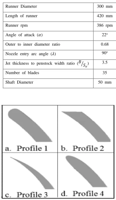
Table 2: Parameters selected for Cross Flow turbines

Runner Diameter 300 mm

Length of runner 420 mm

Runner rpm 386 rpm

Angle of attack (𝛼) 22o

Outer to inner diameter ratio 0.68

Nozzle entry arc angle (𝜆) 90o

Jet thickness to penstock width ratio (𝐵 𝑆⁄ ) 𝑜 3.5

Number of blades 35

Shaft Diameter 50 mm

5

We have selected four different blade profiles for our CFD analysis which are shown in figure 2. Profile 1 has a cir-cular geometry tangent to three sides, 2 blade curves and the D1 of the rotor. Profile 2 is sharp cut at the D1.Profile 3 makes a pointed tip at the inner curve of the blade. Profile 4 has an oval shape with the major diameter twice the minor diameter and the minor diameter equal to the blade thickness.

3. Model Development

The force from the water jet of initial velocity 𝑉𝑖 can be calculated as below, if the blade is considered stationary:

𝐹𝑥= 𝑚 × (𝑉𝑖− 𝑉𝑓𝐶𝑜𝑠𝛼)

𝐹𝑦= 𝑚 × (0 − 𝑉𝑓𝑆𝑖𝑛𝛼)

𝐹𝑦= − 𝑚 × 𝑉𝑓𝑆𝑖𝑛𝛼

Where 𝑉𝑖 : Initial absolute velocity of water

𝑉𝑓 : Final absolute velocity of water

m: mass flow-rate of water α = blade angle

Whereas the resultant force is calculated as follows:

F = √Fx2+ Fy2 F = √[m × (Vi− Vfcos ∝)]2+ [m x Vfsin ∝]2 F = m × √𝑉𝑖2+ 𝑉𝑓2𝑐𝑜𝑠2𝛼 − 2𝑉𝑖Vf𝑐𝑜𝑠𝛼 + Vf2𝑠𝑖𝑛2𝛼 F = m × √𝑉𝑖2+ 𝑉𝑓2(𝑐𝑜𝑠2𝛼 + 𝑠𝑖𝑛2𝛼) − 2𝑉𝑖Vf𝑐𝑜𝑠𝛼 F = m × √𝑉𝑖2+ 𝑉𝑓2− 2𝑉𝑖Vf𝑐𝑜𝑠𝛼 ∴ (𝑐𝑜𝑠2𝛼 + 𝑠𝑖𝑛2𝛼) = 1 F = m × √𝛥𝑉2 _{∴ Δ𝑉}2_{= 𝑉}

6

F = m × ΔV

The power delivered can be calculated as: 𝑃 = 𝐹 × 𝑉

Power delivered to CFT by water will be in two components:

 Firstly, at inlet section of runner

 Secondly, at outlet section of runner

The power produced at inlet section can be calculated as: 𝑇 = 𝑚 × 𝑟𝑉

𝑃1= 𝑇1× 𝑤

Where, 𝑤 = angular velocity of runner

𝑇 = Torque produced by runner shaft

Total power delivered by runner shaft will be:

𝑃 = 𝑃1+ 𝑃2

𝑃 = 𝑚 × [(𝑉1𝑐𝑜𝑠𝛼1) + (𝑉2𝑐𝑜𝑠𝛼1)] × 𝑢1

𝑃 = 𝑚 × [(𝑉1𝑐𝑜𝑠𝛼1) + (𝑉2𝑐𝑜𝑠𝛽2) − 𝑢1] × 𝑢1

The relative velocities of water at inlet and outlet are related as: 𝜈2 = ψ x 𝜈1

Ψ ≈ 0.98 = empirical co-efficient (to neglect the increase in velocity due to difference in height of upper and lower blades)

P = m ((𝑉1𝑥 cos 𝛼1) + (ψ𝜈1𝑥 cos 𝛽2) -𝑢1) x u1

P = m ((𝑉1𝑥 cos 𝛼1) + (ψ×(𝑉1𝑥 cos 𝛼_{cos 𝛽}1)− 𝑢1

1 cos 𝛽2) -𝑢1) u1

P = m [((𝑉1cos 𝛼1) - u1) (1 + (ψ×

cos 𝛽₂ cos 𝛽1 ))] u1

7

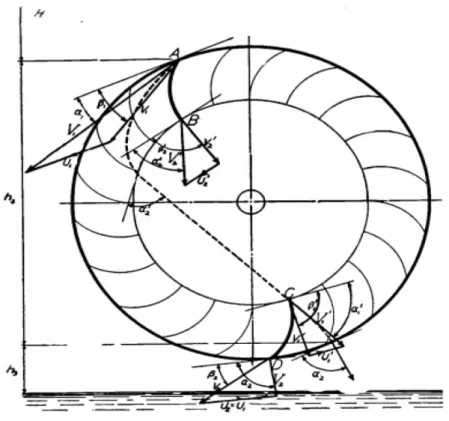
Fig. 3 velocity Triangle

Calculation for Input Power:

The theoretical power input due to head ‘H’ to a CFT can be calculated as: Pi = 𝛾 x Q XH

V1 = C x √2𝑔𝐻

H = 𝑉1

2

2𝑔+ 𝐶2

C = Nozzle discharge co-efficient ̴ 0.98 G= gravitational acceleration

Q = volumetric flow rate of water through CFT runner Suing the above equations

Pi =

𝛾 𝑥 𝑄 𝑥 𝑉₁2 2𝑔 𝑥 𝐶2

8 The efficiency of a CFT will be defined as:

 Ratio of Brake Power to input power due to Head ‘H’.

𝜂 =𝑃

P𝑖

𝜂 =

𝑚 𝑥 [((𝑉1 𝑥 cos 𝛼 1) − 𝑢1) 𝑥 ( 1 + (ѱ 𝑥 cos 𝛽_{cos 𝛽}2

1 ))] 𝑥 𝑢1

𝛾 𝑥 𝑄 𝑥 𝑉12

2𝑔 𝑥 𝐶2

Simplifying the above equation, we get

𝜂 = (2𝐶2𝑥 𝑢1 𝑉1 ) 𝑋 (1 + (ѱ 𝑥 cos 𝛽2 cos 𝛽1 )) 𝑥 (cos 𝛼 1 − 𝑢1 𝑉1)

As the blade angles β1 = β2

𝜂 = (2𝐶2𝑥 𝑢1 𝑉1 ) 𝑋 (1 + ѱ ) 𝑥 (cos 𝛼 1 − 𝑢₁ 𝑉1) It is clear that 𝜂 = 𝑓(𝑢, 𝑉) 𝑢 = 𝑓(𝑟, 𝑤) r = Radius of Runner

w = Angular velocity of Runner 𝑉 = 𝑓(𝐻)

So, 𝜂 = 𝑓(𝑟, 𝑤, 𝐻)

4. Results and Discussion a. ANSYS Analysis

In the current study, the analysis is performed for the different edge profiles of blades for the turbine. The complete turbine is analyzed as the leading edges in the first stage of cross flow become trailing edges in the second stage of the cross flow turbine. For the optimization of blade profiles the second stage cannot be neglected as it has significant power output. For the determination of the most efficient leading and trailing edges, four possible blade profiles are made. The analysis procedure is shown Fig. 4 that consists of CAD model

9

development in CREO 3.0 and then mesh generation in ICEM CFD and finally simulation is carried out in the CFX. The detail methodology of ANSYS analysis is depicted in Fig. 5. In first step, CAD model is developed in the CREO and then CAD geometry is imported in ICEM to edit geometry and named the surfaces. Then mesh is generated and refined. Then the initial and boundary conditions are mentioned. Lastly, the model is solved in the CFX solver and results are generated.

Fig. 4: Flow path for ANSYS Fig 5: Ansys Methodology b. Velocity Streamlines

Velocity streamlines and pressure contours were created in CFD-Post, the following are the results of the simulations. So for simplification we increased the outlet domain so that we have more accurate results and not affecting the ge-ometry of design of the cross flow turbine.

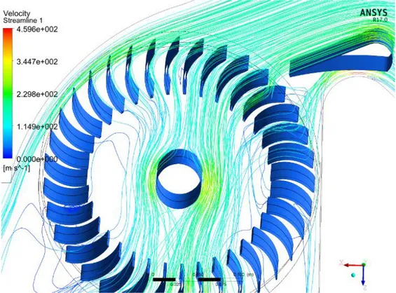
Figures 6, Figure 7, Figure 8 and Figure 9 shows the streamlines in turbine for oval tip blades, round tip blades, pointed tip blades and flat tip blades, respectively. It shows an accurate description of flow in which velocity is increasing in the nozzle and decreasing as it exits the runner and the casing.

CREO Model

Editing the geometry in ICEM CFD Meshing of the Geometry

Exporting the Mesh File

Boundary Conditions and Result Generation

10

Fig. 6: Velocity streamlines for oval tip blades

11

Fig. 8: Velocity streamlines for pointed tip blades

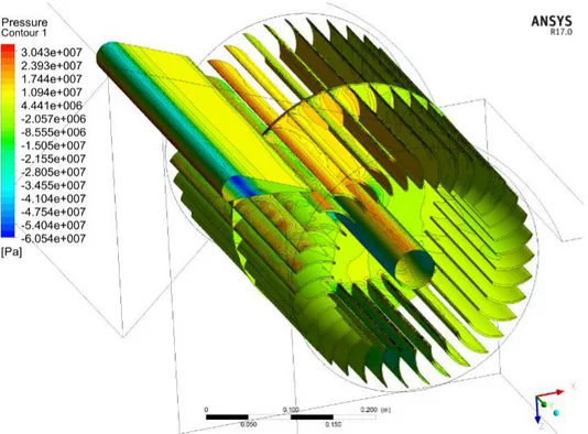
12 c. Pressure Contours

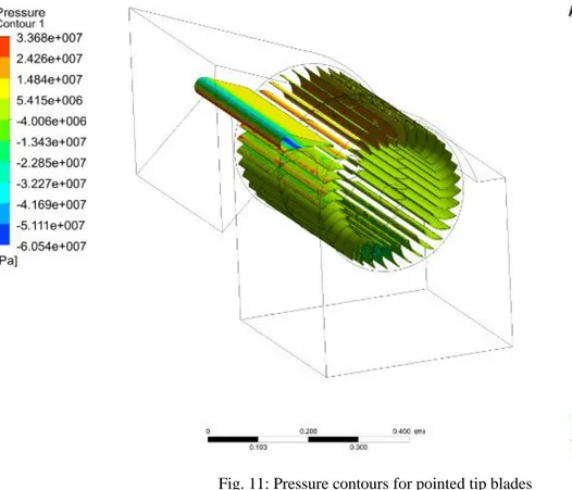
The pressure contours show the variation of pressures along the CFT, pressure decreases as it passes through first stage and further decreases when it strikes the blades of second stage as shown in Fig. 10 for oval tip blades, Fig. 11 for pointed tip blades, Fig. 12 for round tip blades and Fig. 13 for flat tip blade.

Fig. 10: Pressure contours for oval tip blades

13

Fig. 11: Pressure contours for pointed tip blades

14

Fig. 13: Pressure contours for flat tip blades

d. Efficiency Comparison

The simulation was run for the complete turbine and the speed (rpm) was kept constant. All the profiles were simu-lated and tested to elaborated comparison between each profile. The simulation for the four different profiles with the same boundary conditions was done and there results for the simulation were analyzed. The results gave us the toque and using torques, efficiencies for each of the profile was calculated. The comparison of these profiles was done based upon the efficiency. And the conclusion was made regarding which profile is to be used to increase the performance of the turbine. The comparison of the efficiencies for four different blade profiles is shown in table 3. The formulae used for the calculation of efficiencies using total pressure and torque from the ANSYS Results are as follows.

BHP = Torq × W Torq = torque_z()@Blade

15 W = 2×3.142×N/60

IHP = TP × mdot /1000

TP = massFlowAve (Total Pressure) @CASE_IN

mdot = massFlow()@CASE_IN

η = BHP/IHP × 100

Incorporating the above formulae gave us the following the following results for the four Blade Profiles. Table 3: Efficiency (η) of different blades profiles at 386 rpm.

Efficiency

Profile 1 (Round tip) 58.9 %

Profile 2 (Flat tip) 43.8 %

Profile 3 (Pointed tip) 51.4 %

Profile 4 (Oval tip) 53.5 %

5. Conclusion

In this study, cross flow turbine was modeled in CAD CREO software and then simulated in ANSYS-CFX to compare the performance of the CFT for four different blade profiles in terms of their efficiency. The pressure and velocity profiles of four different profiles were computed using CFD tools and then efficiency of four types of pro-files were compared. The results showed that efficiency of the profile-1 (round tip blade) is maximum at same boundary conditions.

6. References

1. Javed Ahmed Chattha, et al. Design of a cross flow turbine for a micro-hydro power application. in ASME

2010 Power Conference POWER2010-27184, July 13-15, 2010 2010. Chicago, Illinois, USA.

2. Javed Ahmed Chattha, M.S. Khan, and A. Haque. Micro-hydro power systems: Current status and future

research in Pakistan. in ASME Power 09 Conference July 21-23, 2009. 2009. Albuquerque, New Mexico,

USA.

3. Dominguez, F., et al., Fast power output prediction for a single row of ducted cross-flow water turbines

16

4. Choi, Y.-D., et al., Performance and internal flow characteristics of a cross-flow hydro turbine by the

shapes of nozzle and runner blade. Journal of Fluid Science and Technology, 2008. 3(3): p. 398-409.

5. Khosrowpanah, S., A. Fiuzat, and M.L. Albertson, Experimental study of cross-flow turbine. Journal of

Hydraulic Engineering, 1988. 114(3): p. 299-314.

6. Nakase Yoshiyuki, et al., A Study of Cross Flow Turbine. Small Hydro Power Fluid Machinery, 1982: p. 6.

7. Totapally, H.G. and N.M. Aziz, Refinement of cross-flow turbine design parameters. Journal of energy

engineering, 1994. 120(3): p. 133-147.

8. FUKUTOMI, J., Y. SENOO, and Y. NAKASE, A numerical method of flow through a cross-flow runner.

JSME international journal. Ser. 2, Fluids engineering, heat transfer, power, combustion, thermophysical properties, 1991. 34(1): p. 44-51.

9. Chiyembekezo S. Kaunda, Cuthbert Z. Kimambo, and T.K. Nielsen1, A numerical investigation of flow

profile and performance of a low cost Crossflow turbine. International Journal of energy and environment

2014. 5(3): p. 21.

10. De Andrade, J., et al., Numerical investigation of the internal flow in a Banki turbine. International Journal

of Rotating Machinery, 2011. 2011.

11. Hydrolink. Hydrolink http://heeco.com.pk/. 2016.

Appendix

Nomenclature

B – Nozzle thickness

D, D1

– External Diameter of Blade

So

- Thickness of jet

H - Head

N’sp

- Specific Speed

t - Blade spacing

HPout

- Output Power

17

u1

- Tangential velocity of Blade outer edge

n - Number of blades

Q - Flow Rate

v1

- Relative velocity of entering water jet

S1

- Tangential blade positioning

u1’ - Tangential velocity of Blade inner edge

V1

- Inlet water jet Absolute velocity

V2’ - Absolute velocity of water from first stage exit

v1’

_Stage)

y1

- Distance of jet from center of shaft

y1

- Distance of jet from inner periphery of the runner

Pt

- Theoretical Power Output

V1’ -

_Stage)

ht

- Head Total

D2

- Inner Diameter of Runner

v2’ - Relative velocity of the water from first stage exit

HPin

- Input Horse Power

C – Coefficient accounting for nozzle roughness

V - Absolute velocity of water along the channel

N - Angular speed of Runner

a - Radial rim width

Greek Symbols:

18

α2’- Angle between the runner inner periphery and absolute velocity of entering water jet

(1

Stage)

β2 -

Angle between the runner periphery and relative velocity of entering water jet (1

Stage)

λ - Nozzle width ratio

ρ - Radius of blades curvature

α1’- Angle between the runner inner periphery and absolute velocity of entering water jet

(2

Stage)

β1

- Angle between the runner periphery and relative velocity of entering water jet (2

Stage)

γ - Specific weight of water

Ѱ - Coefficient accounting for blade roughness

View publication stats View publication stats