ESSAYS ON INDUSTRIAL DYNAMICS: THE CASE OF CHILE

(1)

ESSAYS ON INDUSTRIAL DYNAMICS: THE

CASE OF CHILE

Candidate

Fernando Sossdorf

Internal Commision

Prof. Federico Tamagni

External Commission

Prof. Carlo Pietrobelli

Prof. Werner Hölzl

Supervisor

Prof. Daniele Moschella

International Doctoral Program in Economics

Institute of Economics

Scuola Superiore Sant’Anna

(2)

(3)

List of Figures

1.1 Growth rates distribution, 1995-2006. Pooled data over the period . . . 26

2.1 Horizontal product relatedness density, ISIC Classification . . . 51

3.1 Evolution of market concentration at 7 digits . . . 60

3.2 Evolution of market concentration at 4 digits: sales and employment . . . 61

3.3 Labor Share . . . 62

3.4 Skilled Workers . . . 64

3.5 Contribution to the employment and labor productivity of top firms . . . 73

3.6 Markups . . . 75

3.7 Evolution of the relative price of capital . . . 78

3.8 Evolution of participation index in GVCs . . . 79

3.9 Labor share at the firm level . . . 80

3.10 Labor productivity and purchase of foreign licenses in top 4 firms . . . 81

3.11 Labor productivity evolution and market concentration . . . 82

(6)

(7)

List of Tables

1.1 Heckman estimation: diversification decision . . . 19

1.2 Election of the estimator, growth in employment . . . 20

1.3 Election of the estimator, growth in sales . . . 20

1.4 Diversification and performance: employment growth . . . 21

1.5 Diversification and performance: sales growth . . . 22

1.6 Endogenous switching regression . . . 23

1.7 Treatment and heterogeneity effects . . . 24

2.1 Distribution of HGFs across manufacturing sectors, 1995-2006 . . . 32

2.2 Transition matrix for periods t and t+1 of introducing a new product, 1995-2006 . . . 33

2.3 HGFs in employment and new product introduction . . . 39

2.4 Estimated average partial effects, HGFs in employment . . . 40

2.5 HGFs in sales and new product introduction . . . 41

2.6 Estimated average partial effects, HGFs in sales . . . 41

2.7 Persistence in HGFs in employment and new product introduction, estimated coefficients . . . 42

2.8 Persistence in HGFs in sales and new product introduction, estimated coeffi-cients . . . 43

2.9 Product relatedness in HGFs, estimated coefficients . . . 44

2.10 Natural resource relatedness in HGFs, estimated coefficients . . . 45

2.11 Exclusion restriction in HGFs in employment, estimated coefficients . . . 46

2.12 Unobserved heterogeneity in HGFs in employment, estimated coefficients . . 47

2.13 Redefining HGFs in employment, estimated coefficients . . . 47

2.14 Transition matrix for periods t and t+1, HGFs in employment, 1995-2006 . . 50

2.15 Transition matrix for periods t and t+1, HGFs in sales, 1995-2006 . . . 50

2.16 Summary of studies on HGFs in developing economies . . . 50

3.1 Market Concentration at 4 digits, selected years . . . 60

3.2 Market concentration and labor share . . . 68

3.3 Market concentration and skilled worker share in wage bill . . . 69

3.4 Market concentration and highly skilled worker share in wage bill . . . 70

3.5 Market concentration and labor share: adding imports . . . 70

3.6 Market concentration and highly skilled worker share in wage bill: adding imports . . . 71

3.7 Market concentration and labor share: adding GVCs and price of capital . . . 72

3.8 Market concentration and highly skilled worker share in the wage bill: adding GVCs and price of capital . . . 72

(8)

(9)

Introduction

The thesis investigates the industrial dynamics in the Chilean manufacturing sector. The study of an emerging economy provide a rich theoretical and empirical framework that enriches the analysis of the organizational processes that govern firm activities in these economies.

In this sense, any analysis in developing countries must take into account the specific features of their productive structure (Tybout, 2000; Dutrénit, 2004; Bloom et al., 2010; OECD/ECLAC, 2012; Jensen and Miller, 2018): i) the size of an average firm is very small; ii) firms often do no grow as they age; they enter small and remain small along the firm-life cycle; iii) high differences in relative productivity among micro, small and medium enterprises (SMEs) with respect to large enterprises within and between sectors1; iv) firms in developing countries have low productivity on average relative to firms in advanced economies, v) existence and birth of firms strongly driven by reasons of self-employment in conditions of informality rather than innovative entrepreneurship, and vi) early construc-tion of technological capabilities by the firms reflected in low private indicators of techno-logical effort such as R&D, patents and licenses.

Chile fully complies with the patterns described above. In effect, Chile’s gross domestic product (GDP) has increased substantially in the last two and a half decades, with an aver-age annual growth rate equal to 4.9% from 1990 to 2006 that is the period considered in the thesis, and substantially higher than the average annual global growth (3.4%) during the same period.2

This impressive performance in terms of GDP has not been matched by a structural transformation of the Chilean economy, which is still very similar to a traditional Latin America economy of the 1950s. According to the school of Latin American structuralism (Bielschowsky, 2009), those economies were characterized by three features: i) specializa-tion in primary products and low productive density (low intersectoral complementarity and vertical integration), ii) high differences in labor productivity between and within sectors (structural heterogeneity), iii) institutional structure (State, agricultural sector, en-trepreneurs, among others) with little inclination to investment and technical change. Sev-enty years later, Chile still displays these three characteristics. In terms of sectoral spe-cialization, more than 90% of Chile’s exports in 2015 were primary products and natu-ral resource-based goods, a percentage almost identical to 1962 (91%)3_{. This production}

1_{OECD/ECLAC (2012) shows that the distribution of firms by size is almost equal in Latin America and}

Europe but the productivity of a SME is between 16% to 36% of the productivity of a large enterprise in Latin America, while in Europe this figure is between 63% to 75%.

2_{Data retrieved on September, 2019 from World Development Indicators, World Bank. GDP measured in}

(10)

structure is not usually intense in technological content: 9% of total Chilean manufacturing in 2007 was knowledge-intensive (as measured by the participation of the engineering in-dustries in total manufacturing value added), a percentage even lower than in 1962 (17%) (Cimoli et al., 2010). By way of comparison, the share of engineer-intensive manufacturing in total U.S. manufacturing was 39% in 1962 and 41% in 20074.

Likewise, Infante and Sunkel (2009) using the input-output matrix of the Chilean econ-omy in 2003, show the asymmetric relationship between firms. Small, medium and large enterprises buy almost all intermediate inputs from large firms. In addition, they indicate that in the agricultural sector, a big firm is seven times more productive in terms of la-bor productivity than a small firm, but when comparing the entire agricultural sector with the mining sector in terms of labor productivity, then the latter sector is fifteen times more productive than the agricultural sector. This reveals the low productive density and the structural heterogeneity in which SMEs concentrate all employment and sales but are not the engine of the economy.

A production structure based on natural resources has resulted in that the indicators of effort and technological performance such as the expenditure on R&D over GDP shows poor numbers in Chile in comparison with the advanced economies. In fact, R&D in 2016 amounted to 0.38% of GDP in Chile and 2.74% of GDP in USA5.

Hence, there is a clear dependence of the economy on activities that are not knowledge-intensive. This pattern of specialization has led to a lock-in of the productive structure. In turn, this has had a long-lasting impact on the external and internal gap. The former refer-ring to the technological gap with respect to the developed countries whereas the internal gap lays on the large productivity differences inter and intra-sectors.

In this respect, the thesis is structured in three chapters that seek to respond to this lack of modernization of the Chilean productive structure that is dominated by a few large com-panies that display little innovative behavior, with huge differences in labor productivity between SMEs and large companies, and that also exhibit a high income and wage inequal-ity. For this reason, the thesis try to enrich the empirical literature on firms dynamics in emerging economies (and in Chile) focusing in the following questions: How do firms di-versify? Is there a relationship between diversification and firm performance? Are there high-growth firms in Chile? Is the construction of technological capabilities a key factor for the emergence of these companies? Is there a relationship between changes in market concentration and changes in the labor share? Is there a relationship between changes in market concentration and changes in wage inequality among workers?

Chapter 1 is co-authored with Daniele Moschella. It examines the relationship between product diversification and economic performance at the firm level. As a theoretical frame-work, the resource-view theory explains diversification as the use of underutilized resources within the organization whereas that the capability-based theory establishes that diversifi-cation is understood as an process in that the firm creates, administrates and reconfigure

4_{Data from UNIDO Industrial Statistics Database. Engineering industries correspond to ISIC groups 381,}

382, 383, 384 and 385

(11)

their capabilities. In this sense, product diversification should have a positive effect on per-formance but this relationship may be affected by the direction of diversification, i.e, if it is related or unrelated. At the same time, the decision to diversify has been understood as an exogenous process in many of these studies rather than as a careful strategic decision of a firm. These concerns lead us to estimate a model of diversification of two stages. In the first stage, we model how the firms decide to diversify and how, then, they decide their degree of diversification understood as the relation between the products. The second stage estimate the impact of the degree of diversification on firm growth. As a robustness test, the model is also estimated using a model that consists of only phase: the firms decide to diver-sify and this affect their performance. The results indicate that diversification understood as an endogenous decision affects the firm growth and the model is valid both considering it as sequence of two steps or as a model of one stage.

Chapter 2 is co-authored with Daniele Moschella. It explores as the decision of intro-ducing a new product by a firm affect the probability of having a high-growth episode. Given that firms in the developing economies, in most of the cases, are at an early stage of technological learning, we exploit the introduction of new products as a crucial event in the firm life cycle. In fact, in a stage of early technological development the introduction of new products may play an important role in promoting HGFs. When a firm launches a new good, it diversifies its product range to increase its competitiveness despite the high risks and uncertainties involved in the process. Based on Penrosian theory, a firm’s use of excess production resources should give it a competitive advantage when introducing a new good. This, in turn, should significantly affect the firm growth, which could lead to a high-growth episode compared to other companies that did not change their set of prod-ucts. Using a bivariate recursive probit that considering that the commercialization of a new good is an endogenous decision made by a firm, we find that the launching of a new prod-uct affects positive and significantly the probability of being a HGF. Our results also show that ignoring endogeneity leads to an underestimation of the effect. Once the endogeneity is accounted in the model, the effect of introducing a new good doubles when compared to the baseline model without correction. We also provide evidence that the distance between the product core of the firm and the new product introduced has an additional impact on the probability of being a HGF.

Chapter 3 investigates the effects of product market concentration on labor share and on highly skilled worker share in the wage bill at sector level. In this respect, the impor-tance that a small number of dominant large firms have taken on in the economies has led to a growing interest in the role that these firms might play in the rise observed in mar-ket concentration in advanced economies. One theoretical strand has proposed that this is due to the emergence of superstar firms that have become more efficient with respect to the rest of the firms. This has resulted in a fall in the aggregate labor share due to super-star firms have a lower labor share. In turn, the rise in inequality in the last decades has driven, fundamentally, by the globalization and technological change. The results indicate that a rise in product market concentration is positively associated with a fall in labor share. This is robust even to the inclusion of import penetration and the addition of variables of

(12)

globalization and technological change. Even more, in those sectors where concentration has increased the most, are those where labor participation has fallen the most. In turn, the increase in market concentration is also positively associated with a rise in the highly skilled worker share in the wage bill. But, there is no evidence that Chilean manufacturing firms are superstar firms because they have not become more productive and more inno-vative. On the contrary, they charge a higher markup than other firms, thereby increasing the average markup, leading to an increase in market power. This indicate that a increase in market concentration may be detrimental to the welfare of a country as dominant firms induce wage polarization and increase the market power of the economy.

(13)

Chapter 1

Strategies of diversification and firm

performance

1.1 Introduction

The study of the firms’ dynamics has received considerable attention since the seminal work by Gibrat (1931) which postulate that firm growth is random. This hypothesis has led to a vast analysis of the distribution and determinants of firm growth (Bottazzi and Secchi, 2006; Coad, 2009; Coad and Hölzl, 2010; Gupta et al., 2013). In fact, a general list of the variables most commonly used in empirical studies of the determinants of firms’ growth can be grouped into demographic characteristics such as age and size (Coad, 2016; Haltiwanger et al., 2013), financial (Bottazzi et al., 2014), technological effort (Coad and Rao-Nicholson, 2008) and trade (Grazzi and Moschella, 2017).

As for diversification, different theories have been developed to explain why a firm diversifies. In fact, Castaldi et al. (2003) broadly catalogs four theoretical strand: a market power view, an agency theory, a resource-view and a capability-based theory. The first one is based on the idea that a diversified firm can exert an advantage in terms of power market with respect to a specialized firm. The agency theory postulates that there is a conflict between the managers (agents) and the shareholders in defining the diversification strategy. The resource-view is based on the work of Penrose (1959) in which firm diversification is explained to underutilized resources within the organization. Lastly, the capability-based theory (Dosi et al., 2000) establishes that the firms are characterized by a set of routines, capabilities, which defines their functioning; hence, diversification is understood in this view as an process in that the firm creates, administrates and reconfigure their capabilities. Regarding the link between diversification and performance, a considerable body of research in industrial organization, strategic management, and finance have analyzed the relationship between both variables (Penrose, 1959; Montgomery, 1994; Lang and Stulz, 1994; Berger and Ofek, 1995; Palich et al., 2000). Those studies have found, in general, that the relationship between diversification and performance is non-linear (Palich et al., 2000). In this regard, the relationship is an inverse U-curve in which performance increases at an early stage when firms pass from single-product to multi-product and then decreases at a late stage when multiproduct-firms shift from related to unrelated diversification.

(14)

In turn, the decision to diversify can not be conceived as an exogenous process. In fact, there is a growing empirical literature that has questioned that the diversification is random (Campa and Kedia, 2002; Villalonga, 2004; Brendel et al., 2015). This theoretical strand has postulated that firm scope is an endogenous decision. In addition, empirical literature has used different approaches to measure diversification and its impact on firm growth. This has led to results that are in some cases at odds with theoretical models (Palich et al., 2000). In this sense, our study analyzes the process of diversification in Chilean manufactur-ing. For this purpose, we consider in the analysis, on the one hand, that the diversification process involves a detailed strategy for firms wishing to expand into new lines of business. On the other hand, the relationship between a firm’s growth and the search for new markets can be non-linear. That is, as the company expands its operations it may go into unrelated sectors where the marginal cost of diversifying outweighs the marginal benefit of diversify-ing. In this sense, the analysis incorporates possible non-linearities between diversification and firm growth. Finally, the growth of a company is a multidimensional phenomenon that can yield diverse results depending on the indicator chosen to measure it (Delmar et al., 2003). Indeed, Coad and Guenther (2014) show how the diversification process in Germany affects in different ways the growth in assets employment and sales. Thus, we use employ-ment and sales as measures of growth.

In turn, our work analyzes the diversification process as a process, following Santarelli and Tran (2016) and Dosi et al. (2019), which involves two phases. In the first stage, the firm decides whether to diversify or not. In the second stage, once the firm has diversified, it is estimated how the measure of diversification impacts the firm’s growth. This allows us to study the degree of diversification of a firm understood as the relationship between the products.

Our results provide three insights. First, the decision to diversify is endogenous. In fact, larger, older, export oriented, with a larger proportion of human capital and more capital-intensive firms have a greater probability of diversifying. Second, the degree of di-versification measured by the relationship between the products is affected by this same set of variables. Secondly, once we consider the endogeneity of diversification it has a positive effect on both employment and sales growth. In turn, we find that there is a non-linear relationship between diversification and growth. The additional benefit of diversification is negative so we found an inverted U-shaped relationship. Thirdly, if we consider a direct relation between the diversification process and performance we found that a diversified firm has a higher growth than if it had not diversified but also shows, interestingly, that a firm that did not diversified would have a greater performance in terms of growth if it had. The rest of the paper is organized as follows. Section 1.2 describes the data used in the paper along with the construction of variables. Section 1.3 presents the empirical model to be estimated. Section 1.4 shows the main empirical results. Section 1.5 examines robustness check. Section 1.6 provides concluding remarks.

(15)

1.2 Data and Variables

The data come from the annual national manufacturing census (ENIA) that is described in Appendix: Data Construction. We use form 1 and form 3 to perform our analyses.

We also apply data-cleaning procedure to the data. We exclude firms with missing in-formation, zero or negative values on sales, employment and ISIC code in the form 1. We also eliminate firms in form 1 and 3 where the growth of a variable jump by a factor of 4 or more. Regarding the F3 survey, we drop firms with missing, zero or negative values on sales and/or product’s quantity.

1.2.1 Diversification

Diversification is understood as the business strategy that firms pursue when they operate in different product markets (Ansoff (1958)). In this sense, diversification has been mea-sured in different ways in the empirical literature (Gollop and Monahan, 1991) but the most common election in these studies is the entropy index:

Entropy Indexij= m

∑

j=1 Pj·Ln( 1 Pj )

Pj is the market share of product j for firm i. While Ln(1/Pj)is the weight assigned to each product. For each firm in each year we compute this measure using the form F3 at 7 digits. This indicator is equal to 0 if the firm sells only one product but grows monotonically. Basically, the entropy index measures the relationship between the products of a firm.

1.2.2 Firm growth

Firm growth is defined as a multidimensional process. This means that we compute the one year growth rate in employment and sales as our measures of firm growth:

Growth Empi,t= Ln(Employmenti,t) −Ln(Employmenti,t−1) Growth Salesi,t =Ln(Salesi,t) −Ln(Salesi,t−1)

The growth rate distribution for both variables is shown in Figure 1.1 in the Appendix Figure. As in previous studies (Bottazzi and Secchi, 2006; Coad, 2009), we find that the em-ployment and sales growth rates follows a "tent-shape" distribution. Thus, both variables display fatter tails than a Gaussian distribution. Thus, the entire mass of firms experience almost zero growth but in the left (right) tail there are firms that have greater episodes of rapid (low) growth than their peers.

1.2.3 Control variables

(16)

1. Age: we define the birth of a plant as the first time that appeared in the survey. We computed then the age of the plant as the difference between the current year of opera-tion and the constituent year. Since the dataset spans from 1979 to 2006, the maximum age corresponds to 28 years.

2. Size and Size Squared: measured by the natural logarithm of the total number of em-ployees or the total sales depending in the growth indicator chosen in the regression. 3. Investment intensity: is the division between the capital over the number of

employ-ees.

4. Share of skilled workers: those group of workers are computed as the sum of man-agers,specialized employees and administrative personnel over the total workforce. 5. Dummy Export: this variable is equal to 1 if the plant exports and 0 otherwise.

1.3 Methodology

1.3.1 Modelling the diversification decision

First, we model how the firm decides diversify. In this sense, we created a dummy equal to 1 if the firm is a multiproduct (Dummy MP) in the year t. When a firm diversifies it affects its degree of diversification (entropy index). Thus, the model is as follows

Entropyit=α·Xit+γ·Mit+eit Mit=

(

1 i f Zit·β+ηit> 0 0 i f Zit·β+ηit≤ 0

Where Mitis equal to 1 if the firm is multiproduct and 0 otherwise and the control vari-ables are those defined in the previous section. Since the estimated model corresponds to a Heckman that includes a equation of selection, we must incorporate an exclusion variable that affects the probability that a firm decides to diversify but not its degree of diversifica-tion. Hence, as an exclusion restriction in the selection equation we use the fraction of firms that diversify (FIP) in the same three digit sector but in a different four digit sector in the same way as it is done by Coad et al. (2017).

1.3.2 Degree of diversification and performance

Once the firm has decided to diversify, it chooses its degree of diversification as measured by the entropy index. This, in turn, leads to an effect on the firm’s growth as measured by the following equation:

(17)

Where Growthi,t corresponds to the growth rate of firm i in dimension j (sales or em-ployment) between t−1 and t. Entropyi,tis our diversification measure and Xi,t−1are the control variables. Note that we allow for correlation between the past growth in the future growth. This implies that the model is dynamic panel.

Under the dynamic model, estimation has to take into account the unobserved hetero-geneity and the dependent variable lagged as an explanatory variable. The choice of the OLS estimator will deliver inconsistent estimators independently if T or N grow in the panel (Baltagi, 2002). Whitin Group (WG) also delivers inconsistent estimators (Nickell, 1981) but it is worth mentioning that if T grows, this estimator is consistent. On the other hand, the GMM estimators of Arellano and Bond (1991) and Blundell and Bond (1998) are frequently used in the estimation of dynamic panels. In the case of Arellano and Bond (1991), the model is differentiated and the dependent variable lagged in several periods is used as in-strument to solve the endogeneity given by such variable. However, this GMM estimator has drawbacks if there is high persistence in the data, i.e., if the coefficient of the lagged dependent variable is close to one, leading to bias of the parameters in finite samples or if the ratio of the variance of the individual specific effects to the variance of the idiosyncratic errors is large.

In this sense, Blundell and Bond (1998) add additional moments to do the estimator more efficient. This estimator that consists of moments in difference and in level is known as the "System GMM" estimator. However, Hayakawa (2006) points out that when T and N are large, the instruments used can be inconsistent. In addition, Bun and Kiviet (2006) and Hayakawa (2005; 2006) point out that if the ratio of the variance of individual effects to the variance of idiosyncratic errors is large, the System GMM estimator will present severe deficiencies in estimation.

Flannery and Watson (2007), on the other hand, compare a long list of estimators for dynamic panel (among them fixed effects, OLS, Arellano-Bond GMM and System GMM) for the case of balanced and unbalanced samples under Monte Carlo experiments, with different sample sizes and with a wide variation of the set of parameters given. In the case of unbalanced panels, they find that it is necessary to distinguish between slightly unbalanced or severely unbalanced samples.

Therefore, we will have that our estimator will be based on an adequate choice of the lag for the dependent variable, for which we follow Bond (2002). After choosing the lag, we proceed to settle the most appropriate estimator by means of an experiment of Monte Carlo1with simulated data that replicate our sample. In this way, our first stage investigates the election of the lag for which it is necessary to indicate that the inherent biases of the estimator OLS and Within Group serve for a test of the correct specification of the model. Thus, the OLS estimator is biased upwards so it constitute the upper level of bias of the estimators, while the Within Group estimator is biased upwards. The GMM estimators would be in the middle of both and would be consistent estimators.

(18)

1.4 Results

1.4.1 Diversification decision

The results for the equation of diversification using Heckman are shown in Table 1.1. We have four columns because the first two columns correspond to the model where the size of the firm is measured how the number of employees. Instead, the last two columns measure the size of the firm in terms of sales. For both model, the results show that the diversification process is endogenous. In fact, the likelihood ratio test has a p value equal to 0. It means that the hypothesis that the two parts (main equation and selection equation) are independent can be rejected. Under the logic of the model, it implies that the firm first decide to diversify and the chooses the degree of diversification.

As for the determinants, larger, older, export-oriented, more human capital-intensive and more capital-intensive companies are more likely to diversify both when we consider the size of the company in sales and in employment.

1.4.2 Diversification and performance

Once we find firms decide to diversify and this affects their degree of diversification, the next step is to analyze how the entropy index that measures diversification affects the growth of the company.

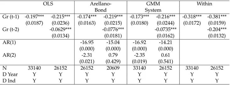
First, Table 1.2 and Table 1.3 show the choice of the lag for employment and sales growth. That is, since we have a dynamic model we must choose the lag of the dependent variable. The OLS and Within Group estimators are the estimators that guide the election of the final estimator because both estimators are biased. For both growth indicators we have that the number of lags is equal to 2. This is because with 2 lags, the GMM system estimator is in the middle of the OLS estimator and the Within estimator. At the same time, with 2 lags we have that the autocorrelation tests of Arellano Bond meet the condition of no having second order autocorrelation.

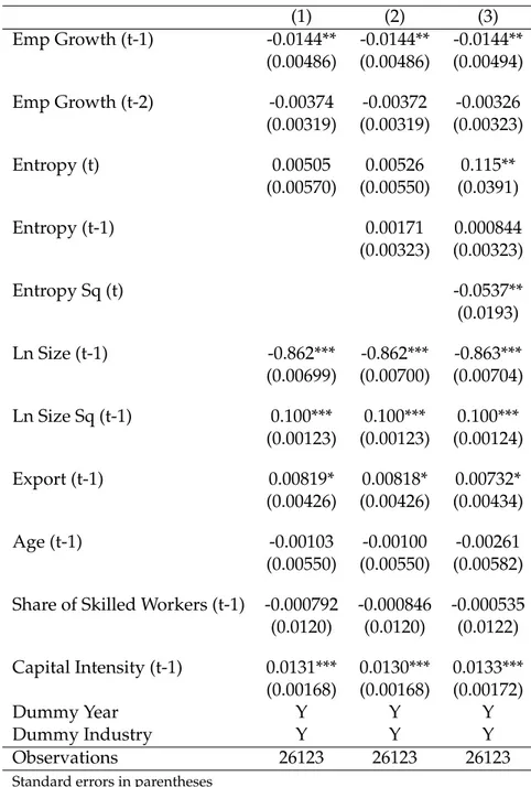
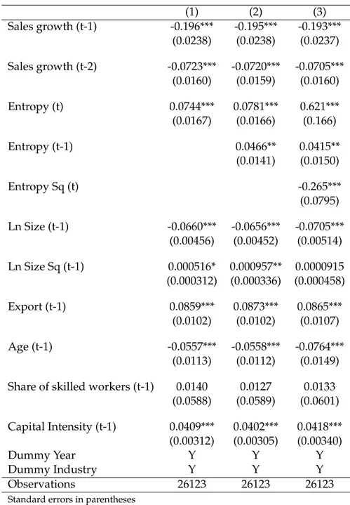
The Table 1.4 and Table ?? show, in turn, the GMM system estimator applied to the equation of employment growth and sales growth. For the employment equation we have that when we only consider the contemporaneous effect of diversification, the effect is pos-itive but not significant. When we add the past value of the diversification variable, the result is still positive but not significant. But, under the general model that includes the quadratic term for capturing non-linearities, diversification impact positively and with a statistically significant coefficient on employment growth. In turn, this relationship is an U inverted as is evidenced by the sign of the diversification variable in its squared value that is negative. In the case of sales, the result is even more significant. That is, the first column shows that the contemporaneous effect of diversification is positive and significant. The second column shows that the past effect of diversification positively affects sales growth while the third column shows that the contemporaneous effect and the past effect have a positive and significant effect on sales growth. Again, diversification is found to follow an inverted U since the sign of the diversification variable in its squared value is negative.

(19)

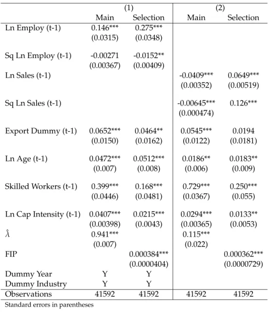
Table 1.1: Heckman estimation: diversification decision

(1) (2)

Main Selection Main Selection Ln Employ (t-1) 0.146*** 0.275*** (0.0315) (0.0348) Sq Ln Employ (t-1) -0.00271 -0.0152** (0.00367) (0.00409) Ln Sales (t-1) -0.0409*** 0.0649*** (0.00352) (0.00519) Sq Ln Sales (t-1) -0.00645*** 0.126*** (0.000474) Export Dummy (t-1) 0.0652*** 0.0464** 0.0545*** 0.0194 (0.0150) (0.0162) (0.0122) (0.0181) Ln Age (t-1) 0.0472*** 0.0512*** 0.0186** 0.0183** (0.007) (0.008) (0.006) (0.009) Skilled Workers (t-1) 0.399*** 0.168*** 0.729*** 0.250*** (0.0446) (0.0481) (0.0367) (0.055) Ln Cap Intensity (t-1) 0.0407*** 0.0215*** 0.0294*** 0.0133** (0.00398) (0.0043) (0.00365) (0.0053) ˆλ 0.941*** 0.115*** (0.007) (0.022) FIP 0.000384*** 0.000362*** (0.0000404) (0.0000729) Dummy Year Y Y Dummy Industry Y Y Observations 41592 41592 41592 41592

Standard errors in parentheses * p<0.10, ** p<0.05, *** p<0.001

1.5 Robustness check

1.5.1 From diversification to performance

One possible critique to the model is that we impose a logic sequence: diversify, choose the degree of diversification and grow. One alternative model can be just the decision of diversification affecting the growth of the firm.

In order to do this, we use a more general framework as is the use of endogenous switch-ing model that has recently been used in the empirical literature by Di Falco et al. (2011), Crowley and McCann (2017) and Coad et al. (2017). Under this specification, firms that di-versify must respond to a particular regime while those that do not must respond to another regime as in shown in the following equation:

(20)

Table 1.2: Election of the estimator, growth in employment

OLS Arellano- GMM Within

Bond System Gr (t-1) -0.154*** -0.163*** -0.130*** -0.166*** -0.136*** -0.170*** -0.278*** -0.355*** (0.0105) (0.0127) (0.0128) (0.0175) (0.0124) (0.0159) (0.0102) (0.0139) Gr (t-2) -0.0531*** -0.0603*** -0.0596*** -0.201*** (0.0109) (0.0144) (0.0142) (0.0114) AR(1) -23.24 -21.36 -23.75 -21.22 (0.000) (0.000) (0.000) (0.000) AR(2) -2.46 0.2 -2.65 0.08 (0.014) (0.839) (0.008) (0.937) D Year Y Y Y Y Y Y Y Y D Ind Y Y Y Y Y Y Y Y N 33140 26152 26152 20609 33140 26152 33140 26152

Table 1.3: Election of the estimator, growth in sales

OLS Arellano- GMM Within

Bond System Gr (t-1) -0.197*** -0.215*** -0.174*** -0.219*** -0.173*** -0.216*** -0.318*** -0.381*** (0.0187) (0.0236) (0.0163) (0.0215) (0.0180) (0.0244) (0.0172) (0.0159) Gr (t-2) -0.0629*** -0.0776*** -0.0735*** -0.204*** (0.0134) (0.0181) (0.0162) (0.0132) AR(1) -16.95 -15.04 -16.92 -14.21 (0.000) (0.000) (0.000) (0.000) AR(2) -2.31 0.79 -2.35 0.61 (0.021) (0.429) (0.019) (0.541) N 33140 26152 26152 20609 33140 26152 33140 26152 D Year Y Y Y Y Y Y Y Y D Ind Y Y Y Y Y Y Y Y

Standard errors in parentheses * p<0.10, ** p<0.05, *** p<0.001 Y_itD =α·X_itD+eD_itY_itND=φ·X_itND+e_itND (1.2) Tit= ( 1 i f Zit·β+ηit>0 0 i f Zit·β+ηit≤0

Where D corresponds to firms that diversify while ND to those that do not. T is the dummy variable equal to 1 if the firm diversified and 0 otherwise. Our variables of control are the same used in the diversification equation.

Under this model, we can compute the average treatment on the treated (ATT) and the average treatment on the untreated (AUT):

(21)

Table 1.4: Diversification and performance: employment growth (1) (2) (3) Emp Growth (t-1) -0.0144** -0.0144** -0.0144** (0.00486) (0.00486) (0.00494) Emp Growth (t-2) -0.00374 -0.00372 -0.00326 (0.00319) (0.00319) (0.00323) Entropy (t) 0.00505 0.00526 0.115** (0.00570) (0.00550) (0.0391) Entropy (t-1) 0.00171 0.000844 (0.00323) (0.00323) Entropy Sq (t) -0.0537** (0.0193) Ln Size (t-1) -0.862*** -0.862*** -0.863*** (0.00699) (0.00700) (0.00704) Ln Size Sq (t-1) 0.100*** 0.100*** 0.100*** (0.00123) (0.00123) (0.00124) Export (t-1) 0.00819* 0.00818* 0.00732* (0.00426) (0.00426) (0.00434) Age (t-1) -0.00103 -0.00100 -0.00261 (0.00550) (0.00550) (0.00582) Share of Skilled Workers (t-1) -0.000792 -0.000846 -0.000535 (0.0120) (0.0120) (0.0122) Capital Intensity (t-1) 0.0131*** 0.0130*** 0.0133*** (0.00168) (0.00168) (0.00172) Dummy Year Y Y Y Dummy Industry Y Y Y Observations 26123 26123 26123

ATT= E(Y_itD|T =1, XD) −E(Y_itND|T=1, XD)AUT= E(Y_itD|T =0, XND) −E(Y_itND|T=0, XND)

(1.3) In fact, we observe E(Y_itD|T=1, XD)and E(Y_itND|T =0, XND)so that E(Y_itND|T=1, XD)

and E(Y_itD|T = 0, XND)are our counterfactual. In addition, we can also compute the base effects (BH) of heterogeneity which tells us that a firm that diversified would have had a higher or a lower growth due to unobserved effects regardless of the fact that a firm diversified and vice versa:

(22)

Table 1.5: Diversification and performance: sales growth (1) (2) (3) Sales growth (t-1) -0.196*** -0.195*** -0.193*** (0.0238) (0.0238) (0.0237) Sales growth (t-2) -0.0723*** -0.0720*** -0.0705*** (0.0160) (0.0159) (0.0160) Entropy (t) 0.0744*** 0.0781*** 0.621*** (0.0167) (0.0166) (0.166) Entropy (t-1) 0.0466** 0.0415** (0.0141) (0.0150) Entropy Sq (t) -0.265*** (0.0795) Ln Size (t-1) -0.0660*** -0.0656*** -0.0705*** (0.00456) (0.00452) (0.00514) Ln Size Sq (t-1) 0.000516* 0.000957** 0.0000915 (0.000312) (0.000336) (0.000458) Export (t-1) 0.0859*** 0.0873*** 0.0865*** (0.0102) (0.0102) (0.0107) Age (t-1) -0.0557*** -0.0558*** -0.0764*** (0.0113) (0.0112) (0.0149) Share of skilled workers (t-1) 0.0140 0.0127 0.0133

(0.0588) (0.0589) (0.0601) Capital Intensity (t-1) 0.0409*** 0.0402*** 0.0418*** (0.00312) (0.00305) (0.00340) Dummy Year Y Y Y Dummy Industry Y Y Y Observations 26123 26123 26123

BH1 =E(YitD|T=1, XD) −E(YitD|T=0, XND)BH2=E(YitND|T=1, XD) −E(YitND|T =0, XND) (1.4) Finally, the transitional heterogeneity (TH) effect indicates if the benefit in terms of growth would have been larger or smaller for those firms that diversified or for those firms that did not.

(23)

Following Crowley and McCann (2017) we use the t-test method to calculate the signif-icance levels for Equations(3) − (5).

Table 1.6 shows that the dummy of diversification is significantly affected by the same variables that affect the firm growth equation. That is, the selection equation indicates that diversification is endogenous. Indeed, larger firms in employment and sales will be more likely to diversify.

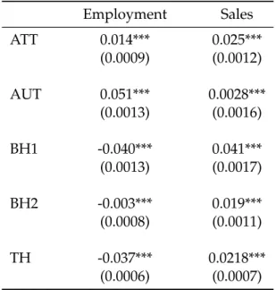
Furthermore, Table 1.7 shows that the treatment and heterogeneity effects are significant for both the employment and sales equation. The second and third columns of the table show that the average treatment effect on the treated is positive and significant. For the employment equation, the magnitude is 1,4% while for the sales growth rate the coefficient is 2,5%. In turn, the average treatment effect on the untreated indicates that there is also a positive and significant effect on both equations. This implies that a firm that did not diversify should have experienced higher employment and sales growth if it had. In fact, a firm that did not diversified but would have done so would have had employment growth of 5,1% and sales growth of 0,3% compared to the current case where the firm did not change its status. This shows that diversification has a positive effect on firm growth.

Table 1.6: Endogenous switching regression

Employment growth Sales growth

Dummy Dummy Selection Dummy Dummy Selection

MP=1 MP=0 MP=1 MP=0

Regime 1 Regime 2 Regime 1 Regime 2 Ln Employ (t-1) -0.14*** -0.10*** 0.12** (0.027) (0.0095) (0.059) Sq Ln Employ(t-1) 0.011*** 0.008*** -0.011 (0.003) (0.001) (0.007) Ln Sales (t-1) -0.34*** -0.25*** 0.17*** (0.048) (0.017) (0.065) Sq Ln Sales (t-1) 0.011*** 0.008*** -0.006** (0.002) (0.0006) (0.002) Export Dummy (t-1) 0.051*** 0.027*** 0.050** 0.034* 0.051*** 0.077*** (0.011) (0.004) (0.025) (0.018) (0.006) (0.024) Ln Age (t-1) -0.016*** -0.010 -0.13*** -0.018** -0.023*** -0.12*** (0.005) (0.002) (0.009) (0.008) (0.003) (0.009) Skilled Workers (t-1) 0.011 0.001 -0.092*** 0.027 -0.007 -0.10*** (0.015) (0.005) (0.032) (0.025) (0.008) (0.031) Ln Cap Intensity (t-1) 0.043*** 0.025*** -0.007 0.034*** 0.020*** 0.007 (0.004) (0.001) (0.008) (0.006) (0.002) (0.008) FIP 3.85*** 0.36*** (0.11) (0.055) Dummy Year Y Y Y Y Y Y Dummy Industry Y Y Y Y Y Y

(24)

Table 1.7: Treatment and heterogeneity effects Employment Sales ATT 0.014*** 0.025*** (0.0009) (0.0012) AUT 0.051*** 0.0028*** (0.0013) (0.0016) BH1 -0.040*** 0.041*** (0.0013) (0.0017) BH2 -0.003*** 0.019*** (0.0008) (0.0011) TH -0.037*** 0.0218*** (0.0006) (0.0007)

1.6 Concluding Remarks

This paper investigates how firm growth is affected by the diversification process. Through a careful methodology of data construction, we have a base that allows us to build a mea-sure of diversification. In this way, we contribute to enriching empirical literature by es-timating how the process of diversification is an endogenous decision that affect the firm growth

Our work presents three main results. This paper investigates how business growth is affected by the diversification process. Through a careful data construction methodology, we have a base that allows us to build a measure of diversification. In this way, we con-tribute to enrich the empirical literature by estimating how the diversification process is an endogenous decision that affects the growth of the company.

Our work presents four main results. First, companies decide diversify or not to diver-sify. Then, they choose their degree of diversification. The diversification decision favors large, more capital-intensive, older and export-oriented firms.

Second, there is a positive and significant effect of diversification on firm growth. This is done by using the diversification measure corresponding to the entropy index through the use of a GMM estimator system that controls by the endogeneity of the entropy index.

Third, the relationship between diversification and growth is non-linear. We find that for Chilean manufacturing, the relationship follows an inverted U as found in other empirical studies. This implies that diversifying is positive at an early stage but at some point it can slow the growth.

(25)

Fourth, even building a model that directly links diversification to growth,we obtain a positive relationship. Moreover, we found that a diversified firm has a higher growth than if it had not diversified but also shows, interestingly, that a firm that did not diversified would have a greater performance in terms of growth if it had.

(26)

1.7 Appendix Figures

Figure 1.1: Growth rates distribution, 1995-2006. Pooled data over the period

1 2 3 4 Log(Pr) −2 −1 0 1 2 x

(27)

Chapter 2

In search of the Chilean jaguar: new

product introduction and high-growth

firms

2.1 Introduction

High-growth firms (henceforth HGFs) have received a considerable attention in recent decades due to the benefits they offer in creating new jobs and promoting economic growth (Henrek-son and Johans(Henrek-son, 2010). In particular, a vast group of empirical studies (see, for a review, Coad et al., 2014 and Moreno and Coad, 2015) have analyzed the determinants of HGFs which notably include demographic factors as size and age, external linkages, localization, financial characteristics and innovative activity.

However, much of these studies have focused on developed countries rather than de-veloping countries. Relatively known is little about the existence and determinants of HGFs in emerging economies as is shown in Table 2.16 in Appendix Tables. A notable exception in this regard is a recent work by the World Bank (Grover Goswami et al., 2018) analyzing HGFs from eleven developing countries: Brazil, Côte d’Ivoire, Ethiopia, Hungary, India, In-donesia, Mexico, South Africa, Thailand, Tunisia, and Turkey. The report shows that HGFs not only contribute substantially to aggregate production and employment, but also that there are strong indirect effects on the firms’ value chain, given the ability of HGFs to in-novate, to create external linkages through exports/imports and foreign direct investment and to attract skilled employment.In addition, they report also explores six determinants that make a firm achieve HGF status: productivity, innovation, managerial capabilities and skills, global linkages and financial development.

The determinants found by the World Bank in its study of 11 emerging economies do not differ much from those found in advanced countries. However, a crucial fact to high-light is that each of these factors is conditioned by the economic development. That is, Bloom et al. (2012) for example, analyzes managerial capabilities in manufacturing firms for several countries being Brazil, China, India and Chile those that exhibit the worst per-formance in management practices. Also, the differences in innovation between countries responds to the construction of technological capabilities that in latecomer firms, following

(28)

the terminology of Dutrénit (2004), are in an initial phase. The latecomer firms are tech-nologically immature, experience a learning process over time, accumulate knowledge and as the technological base expands, create new technologies and develop new products and processes.

In this sense, technological capability is, in our view, one of the crucial factors that may explain the emergence of HGFs in developing economies. Kim (1997), for instance, develops a theoretical framework of the phases of technological learning of an economy in the process of catching up: duplicative imitation, creative imitation and, finally, the innovation phase. Under this setting, many of the firms in these economies focus for a long time on adaptation rather than on the creation of new technologies. In fact, only a small fraction of developing countries have moved into the innovation phase1.

In a stage of early technological development, the introduction of new products may play an important role in promoting HGFs. Indeed, when a firm launches a new good, it diversifies its product range to increase its competitiveness despite the high risks and un-certainties involved in the process. Based on Penrosian theory (Penrose, 1959), a firm’s use of excess production resources should give it a competitive advantage when introducing a new good. This, in turn, should significantly affect the growth of the enterprise, which could lead to a high-growth episode compared to other companies that did not change their set of products.

For this reason, our work analyzes how the introduction of a new product affects the probability of being a HGF in a fast-growth economy as Chile. In this country, the rapid growth in the period 1990-1997 in which GDP grew at an annual rate of 7.7% led a Chilean newspaper, El Mercurio, and scholars (Sznajder, 1996; Montero, 2005) to label the economic miracle as the "Jaguar" of Latin America, echoing the four Asian Tigers and the Celtic Tiger. The excellent macro performance has been reflected also in the firms’ dynamics, as Chilean companies have had an average positive growth and expanded their areas of spe-cialization both domestically and abroad. In fact, one group of Chilean firms have inter-nationalized their operations in Latin America into what has been called the trans-Latin companies (Economic Comission for Latin America and the Caribean (ECLAC), 2013). In turn, an important issue to highlight is that firm diversification in the practice has occurred, generally, in related areas as is suggested by the Penrosian theory.

In this context of high growth at the macro level and at the firm level, HGFs in Chile has been, surprisingly, a scarce area of research (Benavente, 2008; Canales and García Marín, 2018). One fact to highlight, however, is that according to Canales and García Marín (2018) the HGFs represented only 7 percent of the companies, but contributed 40 percent of the jobs created during the 2005-2015 period for the economy as a whole2. This shows the role that HGFs have in promoting job creation in the Chilean economy but leaves open the analysis of which are the determinants that lead a firm to be a HGF.

1_{According to the Global Innovation Index 2018, only China ranks among the top 20 most-innovative}

coun-tries in the world. But, others developing councoun-tries with good innovative performance are Malaysia, Thailand, and Vietnam.

2_{The data in this study come from Chilean Tax authority ( Servicio de Impuestos Internos), and only allow a}

(29)

Our study also incorporates the analysis of the relationship of the new product to the product core. Under Penrosian theory, a firm’s excess of productive resources allows it to produce both related and unrelated goods. However, the direction of diversification is not random but driven by the existing nature of the resources. It means that the introduction of a new product related to the set of products is more favored given the enterprise learning, path dependencies, the selection environment and the existence of complementary assets (Teece et al., 1994). Therefore, we explore whether a product introduced in the same sector as the core of the firm or in sectors not related to the core may have an additional impact on the likelihood of being a HGF. We also evaluate how natural resources sectors introduc-ing natural resources goods in the same sector or in a different natural resource sector may enjoy a additional benefit in terms of reaching a HGF status. This is based on the high de-pendence on natural resources in Latin America in where Chile is a leading case that has led to a lengthy discussion in the region about developing a strategy around them (Ramos, 1998; ECLAC, 2005; Pérez, 2012) or challenge this static comparative advantage by creating dynamic advantages containing Keynesian and Schumpeterian efficiencies (ECLAC, 2012). In this sense, Pérez et al. (2013) argue that Latin America, faced with the wave of ICTs, global production fragmentation and the hyper-segmentation of markets, must exploit the poten-tial of networks around natural resources through the development of specialized niches of high value. In this sense, we explore if there is a natural resources product relatedness among natural resources sectors in Chilean manufacturing firms.

In sum, our paper analyzes as the endogenous decision of introducing a new product is a determining factor in achieving HGF status. Secondly, we also estimate the persistence of HGFs and how the the introduction of a new product by a HGF may have an additional impact on repeating an episode of high-growth. Lastly, we also explore whether product relatedness has an additional impact on the probability of being a HGF. To this end, our research questions are: i) Does the introduction of a new product play a role in the proba-bility of being a HGF?, ii) Is there a persistence in HGFs?, iii) Does the relationship with the product have an additional effect on achieving HGF status?. To consider the endogeneity of the introduction of a new product, we utilize a recursive bivariate probit model.

As a measure of new product introduction, the dataset allows to measure it all new goods produced that are new to the firm but not to the market or the world3. In itself, it is a stricter indicator for evaluating new product innovation, thereby underestimating the value of successful innovations (Cucculelli and Ermini, 2012). However, while these changes to the set of products that only count those new goods introduced for the firm do not consider radical (or breathtaking) innovations as a new good launched into the world, they have a cumulative effect over time that is beneficial to economic growth in developing countries (Puga and Trefler, 2010).

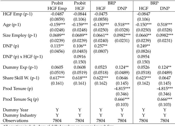
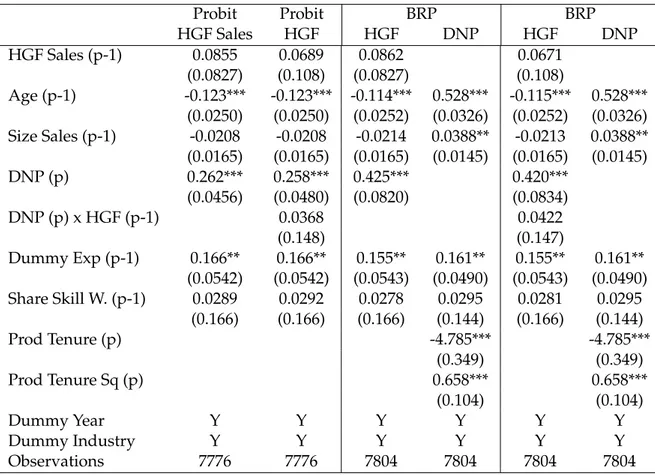
Our results provide five main insights. Firstly, HGFs are present in all sectors. Indeed, there is no over-representation of them in the engineering-intensive sectors. Secondly, the recursive bivariate probit model indicates that the launching of a new good affects positive

3_{It could be also defined as all new goods produced that are new to the firm and the market but not for the}

(30)

and significantly the probability of being a HGF. Estimating the model without endogeneity lead to underestimate the impact of the introduction a new product on reaching HGF status. In fact, when the endogeneity is incorporated to the analysis the coefficient of new product introduction doubles with respect to uncorrected model. Thirdly, there is no persistence of HGFs in statistical terms. A company that was HGF in the previous period decreases its probability of being a HGF in the next period but the coefficient is statistically non-significant. In turn, a firm that was HGF in the previous period enjoys an additional positive benefit when it introduces a new product in the next period but again the coefficient is not statistically significant. Fourth, we find that when a firm introduces a product related to the core of its activities there is no additional effect on the probability of being a HGF. Indeed, there is an additional positive impact when a firm introduces a product not related to its core. This means that when a HGF introduces a product that is vertical or complementary in relation to core, there is a positive and significant effect on the probability of being a HGF. Finally, we find that for HGFs in employment with a core in natural resources, introducing a new good based on natural resources generates a positive and significant impact on the likelihood of being a HGF. Meanwhile, for HGFs in sales the effect is negative and not significant.

The rest of the paper is organized as follows. Section 2.2 describes the data used in the paper and the definition of variables. Section 2.3 presents the empirical model to be esti-mated. Section 2.4 discusses the empirical results. Section 2.5 examines some robustness check and, section 2.6 provides concluding remarks.

2.2 Data and Variables

2.2.1 Sources

The data are obtained from ENIA described in Appendix: Data Construction. The data used comes from forms 1 and 3.

ENIA is available from 1979 to 2015. However, we have information from F3 only from 1995 to 2006. In view of this, our analysis is centered on a panel of firms for this period. Thus, the final sample is composed of 45,476 observations.

2.2.2 Definition of high growth firms (HGFs)

In empirical literature there are two main ways to define high growth firms. On the one hand, one can use an absolute definition of growth. For example, OECD/Eurostat (2007) de-fines HGFs as all firms, starting with at least 10 employees, with average annualized growth greater than 20% per annum over a three year period. Given that the period considered in the analysis includes phases of expansion and recession, the imposition of a growth target of more than 20% may restrict the number of HGFs in recessionary periods of the economic cycle (Guillamón et al., 2017). On the other hand, one can use a relative definition of growth and classify HGFs as those firms in the top X% of the growth distribution (Delmar et al., 2003). Given these two definitions, we choose to use the relative growth of firms given

(31)

that the period considered includes a sharp downturn in the firms’ growth rate due to the Asian crisis but as a robustness check we re-estimate the model using the OECD definition of HGFs.

Once the definition of HGF has been established, a second problem lies in the choice of the growth indicator. Employment, sales, labor productivity, assets, profits and value added are all natural candidates as growth measures for targeting HGFs. For this reason, Delmar et al. (2003) indicate that firm growth is a multidimensional phenomenon as long as HGFs might not grow in the same way along each dimension. In this sense, Daunfeldt et al. (2010) employ nine different definitions of HGFs with low correlation among themselves. In spite of the above, most of the literature has commonly used the employment and sales growth rate as variables to measure firm growth as they are found immediately in the data and can be exchanged as measures of HGFs, given the positive correlation between them, without altering the results overly (Moreno and Coad, 2015). For example, Du and Temouri (2015) use sales growth to define HGFs in their study of the impact of productivity on high growth in the UK while Lopez-Garcia and Puente (2012) use employment growth to characterize HGFs in Spain. On the other hand, Bianchini et al. (2017) and Moschella et al. (2019) define HGFs as those companies that achieve rapid growth in either employment or sales growth. Thus, in the absence of a established framework, we use sales and employment to make a comparison of the HGFs selected under the two definitions. This allows us to compare our results to other studies on HGFs.

As for the time horizon over which to compute growth rates, most empirical studies use periods of 3 to 5 years. This allows to consider HGFs only firms that that grow and sustain their growth over an extended period. That is, a firm in t can have a substantial increase in employment and/or sales but then in t+1 and in t+2 it has a sharp drop in the growth rate of both variables. On the other hand, firms could also increase employment and sales steadily over these three years. Certainly, the second group of firms fits the definition of HGF since there is a continuous rise in sales and employment in the period. Consequently, our analysis for the period 1995-2006 consists of separating it into four phases of similar length (3 years): period 1 (1995-1997), period 2 (1998-2000), period 3 (2001-2003) and, period 4 (2004-2006).

In these four periods, the growth rate of employment and sales is calculated as the log-arithmic difference:

Growth Emp_i,t= Ln(Emp_i,t) −Ln(Emp_i,t−3) Growth Salesi,t =Ln(Salesi,t) −Ln(Salesi,t−3)

Where both sales and employment are normalized by the value at the 3-digits sector in that year to eliminate common trends:

Empi,t =Ln(Empi,t) − ∑ n

i=1Ln(Empi,t) N

(32)

Salesi,t = Ln(Salesi,t) −∑ n

i=1Ln(Salesi,t) N

HGFs are defined in two ways. First, we define as HGFs in employment (HGFe) those firms that are in the top 10% of growth employment distribution in the period. Secondly, and similarly, we define as HGFs in sales (HGFs) those firms that are in the top 10% of the growth sales distribution in the period.

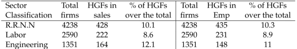
Table 2.1 reports the distributions of HGFs in sales and employment across three broadly defined manufacturing sectors: natural resources-intensive, labour-intensive and engineering-intensive4. This classification is based on Katz, J. and G. Stumpo (2001) who characterize the productive structures of Latin America according to their technological specificities. In the case of Chilean manufacturing, half of firms in the period are concentrated in the natural resources sector, while 17% of firms are in intensive engineering-intensive sectors reflecting a productive structure based on low knowledge-intensive sectors. HGFs are relatively more present in the engineering intensive sector (12.1% and 11%) than in labor or natural resource sector.

Table 2.1: Distribution of HGFs across manufacturing sectors, 1995-2006 Sector Total HGFs in % of HGFs Total HGFs in % of HGFs Classification firms sales over the total firms Emp over the total R.R.N.N 4238 428 10.1 4238 435 10.3

Labor 2590 222 8.6 2590 231 8.9

Engineering 1351 164 12.1 1351 148 11

As for the persistence of the HGFs, there were 154 HGFs in employment and 154 HGFs in sales during the period 1995-1997. In the following period 1998-2000, only 18 firms re-peated their HGF status in employment, and 14 companies maintained their HGF position in sales. Of this group of jaguar companies, in 2001-2003 only 4 held this position in the case of HGFs in employment and 3 in sales. In the period 2004-2006, no HGFs in employment, nor HGFs in sales are able to repeat their status. Thus, there is a small group of jaguar firms that maintain their rapid above-average growth over the period. In fact, the probability that a HGF in employment (sales) in t will repeat its status of jaguar firm in the t+1 is quite low, 12.0% (12.4%), as is shown in Table 2.14 and 2.15 in Appendix Tables.

2.2.3 New product introduction and product relatedness

In order to analyze the relationship between HGFs and new product introduction, we con-struct a dummy of new product introduction which is equal to 1 if the firm produced and sold a new good at the 7-digit in year t and did not produce it in year t−1 or in any previ-ous year, and 0 in another case. This definition is standard in the literature (see, among the others, Cucculelli and Ermini, 2012 and Fernandes and Paunov, 2015a).

4_{Natural resources industries: ISIC groups 311, 312, 313, 314, 341, 351, 353, 354, 355, 362, 369, 371, 372. Labor}

intensive industries: ISIC groups 321, 322, 323, 324, 331, 332, 342, 352, 356, 361, 390. Engineering intensive industries: ISIC groups 381, 382, 383, 384, 385

(33)

As a matter of fact, the average percentage of firms introducing new products over the total is 12.4%. In turn, firms launch only one good in the 95% of the cases and the aver-age turnover over the total sales of the new products is 39.4%. Thus, using a quantitative variable that captures the number of new products produced by a firm adds little infor-mation to the analysis due to the firms seldom produce more of one new good in a given year. Interestingly, however, there is a significant difference in the percentage of news goods commercialized by technological sector in where the average percentage of firm launching new goods in the engineering sector (18.2%) is almost twice as much the natural resources sector (9.5%) while in the labor sector the percentage is equal to 14.2%.

On the other hand, since the calculation of HGFs is done on the basis of a three-year pe-riod, it can be possible that a firm introduces a product each year, in two (non) consecutive years or in just one of those years. In fact, the transition matrix reveals that the commercial-ization of a new product is an infrequent event for the firm: when a firm (not) introducing a new product in t+1 given that plant had (not) introduced a new good in t is obtained a probability of 24.5% (83.6%) as is shown in Table 2.2.

Table 2.2: Transition matrix for periods t and t+1 of introducing a new product, 1995-2006 Period t+1

Not new product Introducing a new product Period t Not new product 83.6 16.4

Introducing new product 75.5 24.5

When a firm introduces a new product, its performance may crucially depends on the "relatedness" between the new product and the core of the firms’ products (see, for example, Piscitello, 2004). On the one hand, a product which is more related to the core may allow firms to exploit economy of scope and increase firm performance (Penrose, 1959; Teece et al., 1994). On the other hand, a product more distant from firm’s main products may open up new growth opportunity (Ng, 2007). In order to investigate the empirical issue of whether more relatedness is good or not in order to be a HGF, we first need to clarify the "relatedness" concept.

Lien and Klein (2009) point out that relatedness measures can be grouped into 3 cate-gories: (i) product distance based on the SIC or ISIC code, (ii) similarity based on the use of inputs from the input-output matrix (IO), (iii) co-occurrence. The first measure is based on the assumption that products in the same ISIC group are related. This indicator assumes that products made in the same sector require similar capabilities for the firm. The second measure uses the input-output matrix to evaluate relatedness not only within the same sec-tor but between secsec-tors in order to capture inter-secsec-toral relatedness. To this end, Fan and Lang (2000) construct an indicator of vertical relatedness to assess vertical integration and an indicator of complementary relatedness based on the assumption that two sectors that use inputs from all sectors of the economy in a similar proportion must be related. The last measure is based on the fact that if, for example, a large number of firms produce goods

(34)

A and B, this indicates a high co-occurrence of the two products reflecting that both goods require similar capabilities for the firms (see, for example, Dosi et al., 2017).

Based on this, we use product distance and similarity based in inputs as measure of product relatedness given that they are the most common measures utilized in the empirical literature (Lien and Klein, 2009) allowing us to compare our results. Hence, we use three measures of product relatedness: i) horizontal; ii) vertical; and iii) complementary. For the calculation of the horizontal relatedness, we first map the classification of products at 7-digits into the standard ISIC classification at 4-digits and then we measure the distance between two products using ISIC at 2-digits. Following Cirera et al. (2011), a new product is considered horizontal related if it is in the same 2-digit product classification as the reference product or firm core. A zero distance means that the new product introduced is related to the core. Figure 2.1 in Appendix Figure shows the horizontal product relatedness density based on ISIC classification at two digits. Most of the observations are clustered around zero indicating that firms introduce product related to their core competencies.

In order to calculate the vertical and complementary relatedness, we use the input-output matrix of the Chilean economy in 2003. Using the correspondence provided be-tween the IO classification and ISIC, vertical relatedness is equal to the average bebe-tween the proportion of input demanded by industry i of industry j and the proportion of input demanded by industry j of industry i while the complementary relatedness is calculated as the correlation coefficient of the input demand of industry i and j with respect to all sectors with the exception of the same sector.

Lastly, the core of the firm is measured as the product with the highest sales in the year t and in the case that a firm introduces more of one product, we compute the distance of each product with respect to the core and then we select the highest value, i.e, the product more unrelated to the core as the measure of product relatedness.

2.3 Methodology

2.3.1 Baseline specification

In our main exercise, we study the effect of the introduction of a new product by a firm on its probability to be a HGF. In order to account for the fact that the introduction of a new product may be an endogenous decision, we use a recursive bivariate probit, RBP (Heck-man, 1978; Maddala, 1983). The RBP is based on a two-equations procedure that allows that the launching of new goods be a dependent binary choice in one equation and an endoge-nous regressor in the other equation. In addition, the RBP also assumes correlation between the errors terms of the two equations and takes into account that unobserved heterogeneity (quality management, leadership, etc) might affect the capacity to introduce a new product by a firm and its capacity to be a HGF. The two equations read as follow:

(35)

Dummy Newpi,p =a+β2·X22i,p−1+c2i+ε2i,p (2.2) In the first equation, HGFj,i,p corresponds to a variable equal to 1 if the firm is HGF according to the definition j (sales, employment) in the period p. Dummy Newpi,p is the variable of new product introduction and X11i,p−1 is a vector that captures a set of control variables. The error term is composed of a firm unobserved heterogeneity (c1i) and an id-iosyncratic error (ε1i,p). As for the second equation,(Dummy Newp)i,pis the variable of new product introduction as a binary dependent variable and X22i,p−1is a vector that captures a set of control variables. The error term is composed of a firm unobserved heterogeneity (c2i) and an idiosyncratic error (ε2i,p). In turn, ε1i,pand ε2i,pare assumed to have a zero mean bivariate normal distribution (Semykina and Wooldridge, 2018).

The recursive bivariate probit can be estimated with the same explanatory variables in both equations (Heckman, 1978; Maddala, 1983). However, in empirical applications one or more variables are added to the second equation to obtain more reliable results (Semykina, 2018). The inclusion of this restriction should be a variable that affects only the probability of introducing a new product but not the probability of being a HGF. In this sense, as an exclusion restriction we exploit the physical characteristics of the products. Hence, the av-erage age of the set of products (product tenure) in each year, as used by Bernard et al., 2010, is added as an explanatory variable in the equation of introduction of new products, and at the same time, we introduce its squared value to detect non-linearity in the relationship (Cucculelli and Ermini, 2012). Thus, the model is initially estimated with an exclusion re-striction and, as robustness check, we test the validity of this rere-striction. As for the common variables for the two equations, they are the following:

• Age: computed as the difference between the current year of operation and the con-stituent year. In turn, the birth of a firm is defined as the first time that appeared in the survey. Since the dataset spans from 1979 to 2006, the maximum age corresponds to 28 years.

• Firm size: measured by the natural logarithm of the total number of employees (sales) when it is used the definition of HGF in employment (sales).

• Share of skilled workers: defined as the sum of managers, specialized employees and administrative personnel over total employment.

• Dummy of exports: equal to 1 if the firm exported in the corresponding year, zero otherwise.

The variable of new product introduction in the period p is equal to 1 if the company launched a new product in at least one year within each three-year sub-period and, zero if not. On the other hand, the control variables at the firm level are measured as an average within each three-year sub-period. In the case of the dummy of exports, this variable is equal to 1 if the firm exported in at least one year within each three-year sub-period and,