Scuola di Scienze
Dipartimento di Fisica e Astronomia Corso di Laurea Magistrale in Fisica
Emulation of neutrino-induced muon
tracks in a neutrino telescope using the
test-bench of the data acquisition system of
the KM3NeT.
Relatore:
Prof.ssa Annarita Margiotta
Correlatore:
Dr. Tommaso Chiarusi
Presentata da:
Francesco Filippini
Oggi l’astronomia multimessaggero offre l’opportunità di investigare, in un modo mai fatto prima, l’universo. In questo quadro l’astrofisica a neutrini e i conseguenti telescopi a neutrini forniscono uno sguardo privilegiato e complementare rispetto alle altre branche di osservazione e nel prossimo futuro permetteranno di gettare luce e di misurare, con estrema precisione, il flusso di neutrini di origine cosmica di alta energia. Questa tesi si sviluppa all’interno dell’esperimento KM3NeT, una rete di rivelatori in costruzione nelle acque abisalli del Mar Mediteranno, che raggiungerà le dimensioni finali di più di un km3 di acqua instrumentata. Nello specifico la tecnologia necessaria alla costruzione
di questi detectors deve essere testata e validata in maniera molto accurata, data la completa inaccesibilità dei siti di installazione. Per questo motivo sono nati diversi laboratori, all’interno della collaborazione, che rappresentano un punto nodale per lo sviluppo, il mantenimento e i test di tutti gli apparati e la strumentazione distribuita in fondo al mare. Fra questi laboratori vi è la Bologna Common Infrastructure (BCI) test-bench, in cui è stata riprodotta l’elettronica e tutto il sistema di acquisizione dati di un’intera stringa di KM3NeT. Questa tesi è basata sul lavoro di sviluppo delle schede OctoPAES, in grado di emulare segnali di fotoni sui fotomoltiplicatori come se fossero stati generati dal passaggio di particelle reali, all’interno però di un ambiente controllato e accessibile come la BCI. Queste schede inoltre sono in grado di generare un flusso di dati manipolabile dall’esterno, capace quindi di evidenziare potenziali malfunzionamenti o punti critici dell’elettronica, del sistema di acquisizione dati e non solo.
Introduction . . . 2
1 Neutrino astrophysics 4 1.1 Neutrino physics and interactions . . . 5
1.1.1 Neutrino interactions . . . 5
1.1.2 Neutrino oscillation . . . 11
1.2 Cosmic rays and atmospheric neutrinos . . . 13
1.2.1 Cosmic ray energy spectrum . . . 14
1.2.2 Fermi acceleration mechanism . . . 16
1.2.3 Acceleration mechanisms above the knee . . . 19
1.2.4 GZK cut-off . . . 20
1.2.5 Acceleration sites . . . 21
1.2.6 Atmospheric neutrinos . . . 23
1.3 Astrophysical neutrinos . . . 25
1.3.1 Neutrino production mechanisms . . . 25
1.3.2 Neutrino and gamma astronomy . . . 27
1.3.3 Neutrino flux . . . 27
1.3.4 State of the art of astrophysical neutrino detection . . . 29
2 Neutrino telescopes and KM3NeT 33 2.1 Detection principle . . . 35 2.1.1 Cherenkov radiation . . . 36 2.1.2 Light propagation . . . 38 2.2 KM3NeT detector . . . 38 2.2.1 Installation sites . . . 39
2.2.2 Digital Optical Module (DOM) . . . 41
2.2.3 Detection Unit (DU) and detector layout . . . 44
2.3 Event signatures . . . 46
2.3.1 Environmental background . . . 50
2.3.2 Physical background . . . 52
3 The Bologna Common Infrastructure test-bench for KM3NeT data acquisition system 54 3.1 Data Acquisition system . . . 55
3.1.1 Control Unit . . . 57
3.1.2 TriDAS . . . 57
3.1.3 Quasi On-Line Analysis and Monitoring system . . . 58
3.1.4 RAW DATA LAN . . . 59
3.1.5 Data handling and timeslice . . . 61
3.2 Algorithms for the event triggering . . . 62
3.2.1 Muon Trigger and reconstruction algorithm . . . 64
3.2.2 Shower trigger . . . 67
3.3 BCI: experimental setup . . . 69
3.4 OctoPAES . . . 72
3.4.1 OctoPAES firmware and wiring topology . . . 74
4 Emulating neutrino induced muon tracks with the OctoPAES boards 85
4.1 Micro-OOS issue . . . 86
4.2 Muon emulation and MIF . . . 90
4.2.1 MIF file . . . 91
4.2.2 GUI for MIF creation . . . 94
4.2.3 Time calibration . . . 101
4.3 Characterisation of the micro-OOS issue at the BCI . . . 104
4.4 Other developments: test with convolutional neural network . . . 107
4.4.1 Regression on zenith angle for neutrino events . . . 110
Conclusions . . . 116
5.1 Summary . . . 116
Introduction
Neutrino astronomy is the youngest branch of astroparticle physics whose aim is to detect neutrino fluxes predicted by various acceleration and propagation models for cosmic rays (CRs). Together with the study of gravitational waves, of CRs and with the detection of gamma-rays, it constitutes the so called multi-messenger astronomy. After 50 years since the proposal by Markov of exploiting deep-sea waters to detect cos-mic neutrinos, IceCube neutrino telescope in the South Pole provided their first ever observation. These recent discoveries allowed to verify and put severe constraints on theoretical models and to assure the effectiveness of the experimental methodology used. The second generation of neutrino telescopes like KM3NeT, IceCube and GVD, under construction or development during these years, has the objective to identify, with a precision never had before, astrophysical sources able to produce high-energy neutrinos and to correlate their direction of flight with gamma-ray or gravitational wave counter-part. In particular, KM3NeT neutrino telescope will reach, in its final configuration, an instrumented volume greater than 1 km3, with hundred of thousands of optical sensors,
becoming therefore the most sensitive high-energy neutrino telescope. In addition, being placed in the Norther hemisphere, it is able to look directly at the centre of our Galaxy, one of the most interesting and promising region where to find neutrino sources.
The thesis is organised as follows:
• the first chapter is focused on the explanation of the physical properties of neu-trinos, of the CR spectrum and of the principal theoretical models today used to explain and predict upper bounds on neutrino fluxes. Also the recent IceCube observations are discussed;
• in the second chapter the detection principle used by neutrino telescopes to de-tect these elusive particles, the physical phenomena affecting the light propagation
and the principal constructive characteristics of the new KM3NeT detectors are exposed;
• in the third chapter the KM3NeT data acquisition system is described with partic-ular attention to its peculiar design and to the trigger algorithms applied to filter the huge amount of data collected. Also, an important part is dedicated to the Bologna Common Infrastructure test-bench and to the introductory works made for the development of the OctoPAES boards;
• in the last chapter the principal objectives and results obtained within the work of this thesis are exposed: the study and development of the OctoPAES boards, the consequent evaluation of the micro Out Of Synchronisation (OOS) issue and the test of Deep Learning frameworks, under construction and development by the KM3NeT collaboration.
Neutrino astrophysics
Neutrino astrophysics is a young discipline, born to extend the conventional astron-omy, based on photons, with the detection of neutrinos, capable to bring completely new information on the source that generate them. During the previous century, great improvements in the survey of the sky came from the enlargement of the detectable elec-tromagnetic spectrum towards the infrared region and with the study of radio emission of peculiar sources. Although these steps forward, that still today produce interesting pictures of the Universe, there are intrinsic limits within this type of observations due to the nature of the photon itself. In fact, it is impossible to observe directly the innermost structure of celestial objects, neither the galactic nuclei that are opaque to photons. Moreover starting at an energy of 10-15 TeV the photons start to interact with the Cosmic Microwave Background (CMB) causing the creation of electron-positron pair. In order to overcome these limits, the study of Cosmic Rays (CRs) and of neutrinos was undertaken, allowing to study the most energetic phenomena occurring in the Uni-verse, through complementary information with respect to what is brought by photons. Furthermore neutrino properties make it a peculiar messenger capable to escape from densest environment without interacting with the Galactic and extra-Galactic magnetic fields. In this chapter the experimental and theoretical status of the high-energy
as-troparticle physics is summed up, with particular attention to neutrino properties and neutrino astronomy.
1.1 Neutrino physics and interactions
Neutrinos are elementary particles, with no electric charge and with spin=1/2. The existence of neutrinos was hypothesized, for the first time, by W. Pauli in 1930 to explain the spectrum of the electrons in the 𝛽-decay [1]. Then four years later, E. Fermi proposed a mathematical theory, in analogy with the electrodynamics (QED), capable to explain the 𝛽-decay, and renamed the particle, previously introduced by Pauli, as neutrino. Only about twenty years later, Reins and Cowan detected the first neutrinos, confirming therefore their existence [2]. Since then, many experimental efforts were carried out, and two further neutrino flavours have been discovered, named muon neutrino [3] and tau neutrino [4]. All neutrino flavours are described within the Standard Model (SM) of particle physics, where they are grouped into three families with the corresponding charged lepton: electron (e), muon (𝜇) and the tau (𝜏). In the SM neutrinos are assumed to be massless, but in order to explain the recent observation of neutrino oscillation [5], the existence of a mass for the neutrino field must be postulated.
1.1.1 Neutrino interactions
The neutrino interaction is described with impressive accuracy within the Standard Model: having electric and colour charge = 0, neutrinos interact only via weak inter-action. The interaction term of the SM electroweak lagrangian for neutrinos can be
explicitly written as: ℒ𝐶𝐶 𝐼,𝐿 + ℒ𝑁𝐶𝐼,𝜈 = − 𝑔 2√2(𝑗 𝜌 𝑊 ,𝐿𝑊𝜌 + ℎ.𝑐.) − 𝑔 2𝑐𝑜𝑠𝜃𝑊𝑗 𝜌 𝑍,𝜈𝑍𝜌 𝑤𝑖𝑡ℎ ∶ (1.1) 𝑗𝜌𝑊 ,𝐿 = 2 ∑ 𝛼=𝑒,𝜇,𝜏 ̄ 𝜈𝛼𝐿𝛾𝜌𝑙 𝛼𝐿 = ∑ 𝛼=𝑒,𝜇,𝜏 ̄ 𝜈𝛼𝛾𝜌(1 − 𝛾5)𝑙 𝛼 (1.2) 𝑗𝑍,𝜈𝜌 = ∑ 𝛼=𝑒,𝜇,𝜏 ̄ 𝜈𝛼𝐿𝛾𝜌𝜈 𝛼𝐿 = 1 2𝛼=𝑒,𝜇,𝜏∑ 𝜈𝛼̄ 𝛾 𝜌(1 − 𝛾5)𝜈 𝛼 (1.3) with 𝑗𝜌 𝑊 ,𝐿 and 𝑗 𝜌
𝑍,𝜈 the leptonic charged current and neutral current terms, 𝜈𝛼 and 𝑙𝛼 the
spinorial field for neutrinos and charged leptons and 𝑊𝜌 and 𝑍𝜌 the two fields associated
with the gauge bosons. Moreover the subscript 𝐿 or explicitly writing the left-handed projector (1−𝛾5)
2 in eq.(1.1) means that weak interaction is maximally parity violating [6],
making interact only left-handed fermions and right-handed antifermions. For further details on SM and weak interaction see [7][8].
Neutrino-nucleon interaction
The interaction processes of neutrinos with ordinary matter are mainly divided into two categories: Charged Current (CC) and Neutral Current (NC), that can be described as follows:
𝜈𝑙+ 𝑋 → 𝑙±+ 𝑌 (𝐶𝐶) (1.4)
𝜈𝑙+ 𝑋 → 𝜈𝑙+ 𝑌 (𝑁 𝐶) (1.5)
with the exchange in the first case of a 𝑊± gauge boson and in the second of a 𝑍0 gauge
boson.
At this point the charged lepton (only in CC channel) and the hadrons, originated from the interaction, can generate an electromagnetic or an hadronic cascade (described in the next chapter).
at-Figure 1.1: Feynman diagram of a generic neutrino-nucleon interaction, producing in the final state a neutral (NC) or a charged (CC) lepton. Attention paid to the kinematical variables. Figure taken from [9].
tention to the kinematics of the process, the following Lorentz invariants can be derived: 𝑠 = (𝑝𝜈 + 𝑝𝑡𝑎𝑟𝑔𝑒𝑡)2 (center of mass energy), (1.6) 𝑄2 = −𝑞2 = −(𝑝
𝜈− 𝑝𝑙)2 (four momentum transferred), (1.7)
𝑦 = 𝑞 ⋅ 𝑝𝑡𝑎𝑟𝑔𝑒𝑡
𝑝𝜈⋅ 𝑝𝑡𝑎𝑟𝑔𝑒𝑡 (inelasticity), (1.8)
𝑥 = 𝑄
2
2 ⋅ 𝑝𝑡𝑎𝑟𝑔𝑒𝑡⋅ 𝑞 (Bjorken scaling variable), (1.9) 𝑊2 = (𝑞 + 𝑝
𝑡𝑎𝑟𝑔𝑒𝑡)2 (invariant hadronic mass) (1.10)
In the lab frame, where the target is at rest, the inelasticity or Bjorken y can be rewritten in this way
𝑦 = 𝐸𝜈− 𝐸𝑙
𝐸𝜈 (1.11)
putting in evidence the physical meaning of this variable: the fraction of neutrino energy transferred to the target. The neutrino-nucleon cross section can be now described in function of the two Bjorken invariants 𝑥 and 𝑦:
𝑑2𝜎 𝐶𝐶 𝑑𝑥𝑑𝑦 = 2𝐺2 𝐹𝑚𝐸𝜈 𝜋 ( 𝑀2 𝑊 𝑄2+ 𝑀2 𝑊 ) 2 [𝑥 𝑞(𝑥, 𝑄2) + 𝑥 ̄𝑞(𝑥, 𝑄2)(1 − 𝑦2)] (1.12) 𝑑2𝜎 𝑁𝐶 𝑑𝑥𝑑𝑦 = 𝐺2 𝐹𝑚𝐸𝜈 2𝜋 ( 𝑀2 𝑍 𝑄2 + 𝑀2 𝑍 ) 2 [𝑥 𝑞(𝑥, 𝑄2) + 𝑥 ̄𝑞(𝑥, 𝑄2)(1 − 𝑦2)] (1.13)
where 𝑚 is the target mass, 𝐺𝐹 ∼ 1.16 × 10⁻⁵ 𝐺𝑒𝑉−2, and 𝑞 and ̄𝑞 are the structure
functions for quarks and anti-quarks. Integrating out the cross sections shown in the previous equations, for neutrino energies above 100 GeV, the following ratio is obtained:
𝜎𝐶𝐶
𝜎𝐶𝐶+ 𝜎𝑁𝐶 ≈ 0.7 (1.14)
This means that the charged current interactions represents around the 70 % of all the neutrino-nucleon interactions.
An interesting and useful approximation is the one in which the target can be consid-ered to be massless. At sufficiently high energies, this is valid for modeling deep inelastic scattering, where the neutrino scatter off a free constituent quark. At the same time, assuming a small four momentum transferred compared to 𝑊± mass and a large centre
of mass energy 𝑠 respect to the mass 𝑚𝑙 of the lepton, the boson propagator effects and
production thresholds, on the cross section calculations, can be neglected. Integrating out the Bjorken variables from eq.(1.13), in the case of neutrino-fermion (equivalent to antineutrino-antifermion) charged current, the differential and total cross section takes this form: 𝑑𝜎𝐶𝐶(𝜈𝑓) 𝑑𝛺 = 𝐺2 𝐹𝑠 4𝜋2, 𝜎𝐶𝐶(𝜈𝑓) = 𝐺2 𝐹𝑠 𝜋 (1.15)
From eq.(1.15) three important observations can be derived:
• cross section depends linearly on 𝑠. If we consider the rest frame of the target, with mass 𝑚, the relation 𝑠 = 𝑚(𝑚 + 2𝐸𝜈) holds, so that the cross section increases
linearly with neutrino energy (E𝜈);
• the cross section grows linearly with the mass of the target 𝑚;
• the cross section doesn’t depend on the neutrino-target scattering angle in the centre of mass frame.
A similar evaluation can be made for neutrino-antifermion (equivalent to antineutrino-fermion) charged current interaction, being careful to the initial helicity states. Due to weak interaction properties we have an initial state with total angular momentum 𝐽 = 1, leading to a preference direction due to angular momentum conservation along the in-teraction axis. The cross section for the process 𝜈𝑙+ ̄𝑓, respect to eq.(1.15), includes an extra factor [1 + 𝑐𝑜𝑠(𝜃∗)]2. In the centre of mass frame the inelasticity 𝑦 is connected to
𝜃∗ with the relation 𝑦 = [1 − 𝑐𝑜𝑠(𝜃∗)]/2. The differential and total cross sections can be
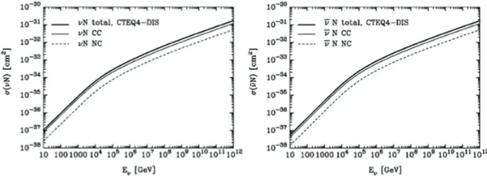
now rewritten in this form: 𝑑𝜎𝐶𝐶(𝜈 ̄𝑓) 𝑑𝛺 = 𝐺2𝐹𝑠 16𝜋2[1 − 𝑐𝑜𝑠(𝜃∗)]2, 𝑑𝜎𝐶𝐶(𝜈 ̄𝑓) 𝑑𝑦 = 𝐺2𝐹𝑠 𝜋 (1 − 𝑦) 2, 𝜎 𝐶𝐶(𝜈 ̄𝑓) = 𝐺2𝐹𝑠 3𝜋 (1.16) Comparing the total cross sections for 𝜈 + 𝑓 and 𝜈 + ̄𝑓 we can see that the second process is suppressed by a factor 3, only for helicity considerations. In Fig.1.2 is shown the behaviour of the total cross section for neutrino-nucleon and antineutrino-nucleon at high energies, in which the dominant process is the deep inelastic scattering [10].
Figure 1.2: left: neutrino-nucleon cross section; right: antineutrino-nucleon cross section. In both, total cross section (bold line), and the single components: CC (solid line) and NC (dashed line) are shown. Figure taken from [10].
Neutrino-electron interaction
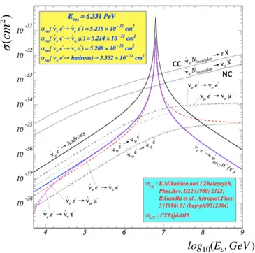
As analysed above, the total cross section is linearly dependent on the mass of the target. This produces a suppression of three orders of magnitude for the neutrino-electron process with respect to the neutrino-nucleon one. This is a general behaviour over a wide energy range, except in a precise interval, 𝐸𝜈 = 5.7 ÷ 7.0 PeV, where it is
present the resonance production of a real W− boson, as in the process: ̄𝜈
𝑒+ 𝑒−→ 𝑊−
[10]. The peak of the resonance, as shown in Fig.1.3 is at an energy around 𝐸𝜈 ∼ 6.3
PeV, and is called Glashow resonance. This process was postulated in the late 1960s
Figure 1.3: The glashow resonance, peaked at an energy around 6.3 PeV.
but still remains unobserved. The biggest challenge is the building of detectors capable to reveal neutrinos at such high energies. Nowadays with the construction of neutrino telescopes, capable to detect high-energy astrophysical neutrinos, observation becomes
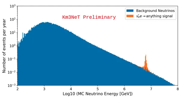
the detection of the process with KM3NeT-ARCA telescope, with one year of observation [11].
Figure 1.4: Expected event rate in one building block of KM3NeT-ARCA after one year of observation. The orange peak corresponds to the Glashow resonance events only. Blue histogram contains all other neutrino interactions in the detector. Figure taken from [11].
1.1.2 Neutrino oscillation
In this section I will briefly describe the neutrino oscillation phenomenon, and its implications on neutrino astronomy. The oscillation of the neutrino flavour originates from the fact that flavour eigenstates do not coincide with mass eigenstates. In fact pure flavour eigenstates, originated from weak interaction processes, are mixture of at least three mass eigenstates with unequal mass. This difference will lead, during the propagation in vacuum, to a periodic change in the probability that a flavour eigenstate 𝛼 will be detected as another flavour eigenstate 𝛽, with 𝛼 ≠ 𝛽. The following section is inspired by [12].
Three family formalism
A neutrino with flavour 𝛼 and momentum ⃗𝑝, created in CC or NC processes, can be described as follows:
|𝜈𝛼⟩ = ∑
𝑘
𝑈∗
𝛼𝑘|𝜈𝑘⟩ , 𝛼 = 𝑒, 𝜇, 𝜏 (1.17)
where |𝜈𝑘⟩ are the orthonormal massive neutrino states and 𝑈𝛼𝑘 is the mixing matrix,
also known as Pontecorvo-Maki-Nakagawa-Sakata (PMNS) matrix [13][14]. The matrix 𝑈 can be parametrized by 3 mixing angles 𝜃𝑖𝑗 and a complex phase 𝛿, encoding the possible CP violation (recent results on 𝛿 value, reported by T2K experiment can be found at [15]): 𝑈 = ( 1 0 0 0 𝑐23 𝑠23 0 −𝑠23 𝑐23 )( 𝑐13 0 𝑒𝑖𝛿𝑠 13 0 1 0 −𝑒𝑖𝛿𝑠 13 0 𝑐13 )( 𝑐12 𝑠12 0 −𝑠12 𝑐12 0 0 0 1 ) (1.18)
The unitarity of the mixing matrix 𝑈 transposes the mass eigenstate orthonormality property also to the flavour eigenstates:
⟨𝜈𝛼|𝜈𝛽⟩ = 𝛿𝛼𝛽 (1.19)
In eq.(1.17) it is not set an upper limit on the number of massive neutrino states. The number of active flavour neutrinos is three, so the number of massive neutrino states must be grater or equal to three. However, the massive neutrino states are eigenstates of the Hamiltonian ℋ, with eigenvalue 𝐸𝑘, with energy given by the usual relativistic
dispersion relation. Therefore the Schröedinger equation can be written: 𝑖𝑑
𝑑𝑡|𝜈𝑘(𝑡)⟩ = ℋ |𝜈𝑘(𝑡)⟩ (1.20)
that gives us, as result, the usual evolution in time of the neutrino mass eigenstates as plane wave. At this point the time evolution of flavour eigenstates is given by:
|𝜈𝛼(𝑡)⟩ = ∑𝑈∗
Considering the initial condition |𝜈𝛼(𝑡 = 0)⟩ = |𝜈𝛼⟩, and eq.(1.17), the evolved flavour eigenstate, at a generic time 𝑡 in function of the initial flavour eigenstate, is given as follows: |𝜈𝛼(𝑡)⟩ = ∑ 𝛽=𝑒,𝜇,𝜏 ( ∑ 𝑘 𝑈𝛼𝑘∗ 𝑒−𝑖𝐸𝑘𝑡𝑈 𝛽𝑘) |𝜈𝛽⟩ (1.22)
The probability of the transition 𝜈𝛼 → 𝜈𝛽, as a function of time can be written in this
form: 𝑃𝜈 𝛼→𝜈𝛽(𝑡) = |𝐴𝜈𝛼→𝜈𝛽| 2 = ∑ 𝑘,𝑗 𝑈∗ 𝛼𝑘𝑈𝛽𝑘𝑈𝛼𝑗𝑈𝛽𝑗∗ 𝑒−𝑖(𝐸𝑘−𝐸𝑗)𝑡 (1.23)
For ultra-relativistic neutrinos the relation 𝐸𝑘− 𝐸𝑗 ∼ 𝛥𝑚2𝑘𝑗
2𝐸 holds, and the propagation
time can be replaced with the distance between the source and the detector L (𝑡 = 𝐿 in natural units) leading to:
𝑃𝜈𝛼→𝜈𝛽(𝐿, 𝐸) = ∑ 𝑘,𝑗 𝑈𝛼𝑘∗ 𝑈𝛽𝑘𝑈𝛼𝑗𝑈𝛽𝑗∗ 𝑒𝑥𝑝( − 𝑖𝛥𝑚 2 𝑘𝑗𝐿 2𝐸 ) (1.24)
The amplitude of the oscillation is specified by the elements of the mixing matrix, while the phase of the oscillation is determined by the square mass differences 𝛥𝑚2
𝑘𝑗. The
neutrino oscillation produces a change in the ratio of neutrino flavours, when propagates towards the detector. In fact neutrinos produced in astrophysical environments, from 𝜋 or 𝐾 decay have a ratio 𝜈𝑒 ∶ 𝜈𝜇 ∶ 𝜈𝜏 = 1 ∶ 2 ∶ 0 at the source, which is changed during
the path. At Earth is expected to be 𝜈𝑒 ∶ 𝜈𝜇 ∶ 𝜈𝜏= 1 ∶ 1 ∶ 1.
1.2 Cosmic rays and atmospheric neutrinos
The Cosmic Rays (CRs) are an isotropic flux of protons and heavier nuclei hitting the upper shell of the Earth atmosphere. The name “Cosmic Rays” was used for the first time by Robert Millikan in 1925, after several studies and experiments carried out, since the beginning of the century, by V.F. Hess. Although the study and knowledge on
CRs have advanced a lot in the last century, there are however still some open questions on the nature and the source that generates these energetic particles. In fact, being mainly composed by protons, having an electric charge = +1, they interact with the Galactic and extra-Galactic magnetic fields, making back-propagating the particle to its source impossible. Therefore, during the years, other methods and other messengers, like neutrinos, were studied in order to put constraints and gather some complementary information on the source that generate them.
1.2.1 Cosmic ray energy spectrum
The energy spectrum of primary cosmic rays, shown in Fig.1.5, measured through direct and indirect techniques spans from ∼ 109 eV to more than 1020 eV, is of
non-thermal origin and follows a broken power law [16]: [𝑑𝑁𝑃
𝑑𝐸 ]
𝑜𝑏𝑠
= 𝐾𝐸−𝛼 (𝑐𝑚−2𝑠𝑟−1𝑠−1𝐺𝑒𝑉−1) (1.25)
Fitting the experimental points with the power law written above, we obtain 𝛼 = 2.7 for energies below 3 × 10¹⁵ eV. Above this value, the spectral index become 𝛼 = 3.1:
this change in spectral index is also known as knee. At energies of the order of 1019
eV, the spectrum flatten again, reaching an index 𝛼 = 2.7 and this feature is called
ankle. The acceleration of CRs and the consequent spectrum measured at Earth can
be explained through different models and acceleration mechanisms: till the knee the longest-established model is the Fermi acceleration mechanism, discussed in the next section. There are instead still lots of uncertainties on the acceleration mechanisms at energies between 1015 eV and 1019 eV. After the ankle, considering the energy of
the CR and the mean value of the Galactic magnetic field ⟨𝐵⟩ ∼4 𝜇𝐺, the Larmor radius can be evaluated and compared to the longitudinal and transversal dimensions of our Galaxy, reaching the conclusion that this part of the spectrum has an
extra-Figure 1.5: CRs differential energy spectrum, measured from multiple experiments. Note that the spectrum is remarkable continuous over the whole energy interval. The black solid line represents a E−3 spectrum. Figure taken from [17]
are shown in Fig.1.6 for different CR energies. Up to energies of 1014eV, the CR spectrum
is directly measured through balloons or satellites, providing also relevant information about the chemical composition of primary CRs. These measurements show that CRs are composed by ∼ 90% of protons, ∼ 9% of helium nuclei and ∼ 1% of heavier nuclei. Above ∼ 1014eV, CR measurements are only accessible from ground detectors, capable to
instrument a large area and reveal secondary particles contained in the shower generated by the interaction of primary CRs with the nuclei in the atmosphere. The difficulties related to these indirect measurements produce still some uncertainties on the precise
Figure 1.6: Simulated trajectory of CRs in the Galactic magnetic field. The three different energy regimes are chosen to put in evidence how CRs at energies ∼ 1019 eV
travel along almost straight lines and are not trapped inside the galaxy.
determination of the chemical composition of CRs. For this reason in Fig.1.5 the CR spectrum is summed over all the possible mass numbers of primary CRs, resulting in an
all-particle energy spectrum.
The content of the next section is get inspired by [18].
1.2.2 Fermi acceleration mechanism
The Fermi acceleration mechanism, formulated for the first time by E. Fermi in 1949 (second-order Fermi mechanism) [19], and corrected in 1954 (first-order Fermi mecha-nism), is the most accredited model to explain the acceleration of primary CRs till the knee. It explains the acceleration of charged particles in regions with very strong inho-mogeneous magnetic fields. The idea at the base of the model can be easily illustrated using a toy model: two approaching trains. If a ball is thrown from the train B, moving with velocity 𝑉 towards train A, at a speed 𝑣 in the rest frame of the train B, the speed of the ball in laboratory frame will be 𝑣1 = 𝑣 + 𝑉 and 𝑣𝐴1 = 𝑣 + 2𝑉 in the frame of
train A. If the collision is assumed to be elastic, the ball will bounce back with a velocity in the laboratory frame of 𝑣2 = 𝑣 + 3𝑉. Considering the gain in each collision to be
very high energies. Considering now protons or nuclei bouncing back and forth between two consecutive shock waves, originated in environments of disruptive events like stellar gravitational collapses, the similarity with the toy model exposed above can be caught. Considering a relativistic regime, Lorentz transformations need to be applied to go from a reference frame S, the one of the observer, to the reference S’, the one in which the shock wave or the magnetised cloud is at rest. Applying the transformations iteratively, for each collision, the final energy of the particle in the observer frame can be written as:
𝐸∗ ∼ (1 + 2𝑈 𝑣
𝑐2 𝑐𝑜𝑠𝜃 + 2
𝑈2
𝑐2) ⋅ 𝐸 (1.26)
where U is the velocity of the cloud in S frame. The second term is equal to zero when averaged over all the possible directions. Furthermore energy is gained (cos𝜃 > 0) for head-on collisions and lost for catching collisions: in this case the energy gained 𝛥𝐸 ∝ (𝑈 /𝑐)2 (second-order Fermi mechanism). Instead if it is assumed an astrophysical environment in which only head-on collisions occur, the quadratic term in U can be neglected, being 𝑈/𝑐 ≪ 1, and approximate 𝑣 ∼ 𝑐 being in a ultra-relativistic regime. Now averaging the 𝑐𝑜𝑠𝜃 over the range [−𝜋/2, 𝜋/2] in which only head-on collisions occur, we obtain: ⟨𝐸∗⟩ = (1 + 4 3 𝑈 𝑐) ⟨𝐸⟩ ≡ ℬ ⟨𝐸⟩ (1.27) ⟨𝛥𝐸⟩ = (4 3 𝑈 𝑐) ⟨𝐸⟩ ≡ 𝜂 ⟨𝐸⟩ (1.28)
Recollecting now the power law extracted experimentally from the CR spectrum, we need to consider also another factor: Pescrepresenting the possibility that, after a collision, the particle escapes the acceleration region, making it lose the successive iterations. If the mechanism is efficient, the Pesc is small. The probability that a particle remains inside the acceleration region after 𝑘 collisions is (1-Pesc)𝑘, and starting with N
initial energy E0, after 𝑘 collisions there will be:
𝑁 = 𝑁0𝑃𝑘 particles with energy ≥ 𝐸 = 𝐸
0ℬ𝑘 (1.29)
Removing the 𝑘 parameter from previous equation: 𝑙𝑛(𝑁 /𝑁0) 𝑙𝑛(𝐸/𝐸0) =
𝑙𝑛𝑃
𝑙𝑛ℬ (1.30)
the power law required is obtained: 𝑁 (≥ 𝐸) 𝑁0 = ( 𝐸 𝐸0) 𝑙𝑛𝑃 /𝑙𝑛ℬ (1.31) Supernova remnants (SNR) are the most accredited sites of acceleration of CRs in the region up to the knee. Applying the Fermi mechanism to this type of sources, it predicts a spectral index 𝛼 = 2 and fits correctly the energy power of 5 × 1040 erg/s required
to accelerate Galactic CRs till the knee. The apparent tension with the spectral index measured from the CR spectrum (𝛼 = 2.7) can be solved considering the Galactic dif-fusion of CRs, explained in the so called leaky box model [20]. Fig.1.6 shows charged CRs confined by Galactic magnetic fields, having a small probability to escape from the Galaxy itself. Increasing CR energy, the gyromagnetic or Larmor radius will increase, producing a larger probability for the CR to escape. Therefore an energy-dependent diffusion probability P can be defined, and measured experimentally through the ratio between light isotopes (Li, Be, B). It was found P(E)∝ E𝛼𝐷, with 𝛼
𝐷 = 0.6. The final
differential flux of CRs at source is: [𝑑𝑁𝑃 𝑑𝐸 ] 𝑠𝑜𝑢𝑟𝑐𝑒 ∝ [𝑑𝑁𝑃 𝑑𝐸 ] 𝑜𝑏𝑠 ⋅ 𝑃 (𝐸) ∝ 𝐸−𝛼⋅ 𝐸𝛼𝐷 ∝ 𝐸−𝛼𝐶𝑅 (1.32)
There is however some uncertainties on the nature of the knee in the CR spectrum. Some models lead back to astrophysical reasons, and to a dependence of the maximum obtainable energy in the acceleration sites on the nucleus charge 𝑍𝑒. This produces a different cut-off for every nucleus type, resulting in a proton-rich spectrum before the
1.2.3 Acceleration mechanisms above the knee
The Fermi mechanism and SNR models can explain the CR flux till 1016 eV, but
there is no preferred models for explaining the acceleration of CRs till 1019 eV. The
idea is centred on the possibility, for already accelerated CRs, to suffer an additional acceleration due to, for example, neutron star strong variable magnetic field. In fact, in astrophysical environments the matter is in the form of plasma and no static electric fields can be generated. However, thanks to Faraday’s law, variable magnetic fields can produce induced electric fields capable to accelerate charged particles. From simple dimensional arguments, the maximum obtainable energy from a pulsar1 can be derived
[18]: ℰ 𝑅pulsar = 1 𝑐 𝑑𝐵 𝑑𝑡, (1.33) 𝐸max= ∫ 𝑍𝑒ℰ𝑑𝑥 = ∫ 𝑍𝑒𝑅pulsar 𝑐 𝑑𝑥 𝑑𝑡𝑑𝐵 = 𝑍𝑒𝑅pulsar𝐵 𝜔pulsar𝑅pulsar 𝑐 (1.34)
Replacing the estimated values for the pulsar angular velocity 𝜔pulsar and radius 𝑅pulsar, we obtain:
𝐸max ∼ 5 × 10⁶𝑒𝑟𝑔 ∼ 3 × 10¹⁸𝑒𝑉 (1.35)
Even if a small part of the total rotational energy of a single pulsar can be used to generate the entire power required from CR flux in the energy range knee-1018 eV,
theoretical details on the mechanisms are still not known. Another model that tries to explain the acceleration of CRs in this energy range exploits binary systems and still huge variable magnetic fields. These fields are produced by the huge amount of ionised
1Pulsar is a rotating neutron star that emits a beam of electromagnetic radiation, typically along its magnetic axis. From simple arguments like angular momentum conservation, we can derive typical angular velocity and magnetic field of this object: 𝜔pulsar=12 500 rad/s, 𝐵pulsar∼ 1012G. Nowadays more than 2600 pulsar are known.
matter that falls from one object to the other, transforming in this case gravitational energy into electromagnetic energy and then in acceleration of charged particles.
1.2.4 GZK cut-off
With the discovery of the Cosmic Microwave Background(CMB), in 1966, indepen-dently G. Zatsepin, V. Kuz’min,[21] and K. Greisen [22] hypothesised the suppression of the Ultra High Energy Cosmic Rays (UHECRs) flux, due to the resonant production of pions in the interaction of protons with the CMB, through the following processes:
𝑝++ 𝛾
𝑐𝑚𝑏 →𝛥+→ 𝑛 + 𝜋+ (1.36)
𝛥+→ 𝑝 + 𝜋0 (1.37)
𝛥+→ 𝑝++ 𝛾 (1.38)
The neutral pions decay into gammas, while the charged ones decay mainly into 𝜇+𝜈.
The decay of the neutron into a 𝑝 𝑒 ̄𝜈𝑒 produces, in all the final states, a proton with
reduced energy due to the simultaneous pion production. What is expected therefore, is the suppression of the proton flux for energies above 𝐸 ∼ 5 ⋅ 1019 eV, value obtained
from kinematics considerations. This suppression is also known as GZK-cutoff. Also the
energy loss length 𝑙𝑝𝛾 can be estimated:
𝑙𝑝𝛾 = 1
⟨𝑦 𝜎𝑝𝛾 𝑛𝛾⟩ =
1
0.1 ⋅ 250 × 10−30⋅ 400 = 1026𝑐𝑚 = 30𝑀 𝑝𝑐 (1.39)
where 𝑦 is the Bjorken variable, introduced in the previous section. All protons originated at distances larger than ∼30 Mpc from the Earth, are energy suppressed due to this effect. The estimate of the chemical composition of CRs, even at such high energies, is fundamental to confirm the existence of the GZK cut-off: in fact for heavier nuclei, with mass number A and energy E, the resonance production occurs through the interaction of a nucleon of energy E/A within the nucleus with the CMB. The threshold energy for
already reported some interesting results [23] that shed some light on the composition of CRs in the most energetic part of their spectrum, but better resolution and improvements are expected in the next future.
1.2.5 Acceleration sites
Nowadays we know several sites where the acceleration of primary CRs may occur. In the following some are listed [16]:
• Supernovae Remnants (SNR): these are the most accredited sites responsible for the acceleration of CRs up to the knee, through Fermi mechanism. At the be-ginning of the collapse of a core-collapse or type II supernova, the reaction of electron capture on protons inside Fe nuclei is energetically favoured, producing neutron-rich nuclei in the core of the collapsing star. Some of the nuclei decay through 𝛽-decay producing a large fraction of ̄𝜈𝑒. These particles are trapped in-side the star due to high density reached in the process. When the core of the star reaches the nuclear density (𝜌 ≈ 1014 g/cm3) the in-falling material bounces
back, producing a shock wave that triggers the supernova explosion. The nascent remnant will evolve into a neutron star or into a black hole, depending on the mass of the progenitor, above or below ∼25 solar masses. ̄𝜈𝑒 produced in the early
stages are now capable to escape, causing the neutrino burst. 99% of the gravita-tional energy (3 × 1053 erg) is carried away by neutrinos, and only the remaining
1% is subdivided among photons and kinetic energy transferred to the expand-ing material, resultexpand-ing however to be the perfect location for the acceleration of CRs. Most of the neutrinos are emitted with a thermal spectrum, with a mean energy around 15 MeV. The energetic balance is one of the most important ar-guments as proof of the acceleration mechanism in this type of sources. In fact considering the kinetic energy emitted (∼ 1051 erg) and the number of observed
erg/s, comparable to the power lost by the Galaxy itself through propagation and escape of CRs, resulting therefore in a stationary condition. Recent observations in gamma-ray astronomy by HESS collaboration [24], show strong evidence and also morphological characterisation of the production of gamma-rays in the SNR named RX J1713.7−3946;
• Pulsar wind nebulae (PWNe): also called Crab-like remnants, it is a SNR that dif-fers from the previous one because a pulsar is present in the centre blowing winds and jets of material in the surrounding nebula. The radio, X and optical obser-vations suggest an origin of the electromagnetic component through synchrotron radiation, even if an hadronic origin, with subsequent neutrino emission, is not still discarded. The neutrino flux calculated, thanks to the constraints imposed by gamma observations, for this type of sources can be detected by a km3 neutrino
telescope;
• Microquasar: they are binary systems, emitting jets of relativistic particles re-vealed in the radio band. They result morphologically similar to AGN (see in the following) and are generally formed by a black hole and by an orbiting star that donates the material for the jets. They are considered to accelerate particles up to ∼ 1016 eV.
While the previous sources are typically acceleration sites within our Galaxy, the most energetic part of the CR spectrum seems to have an extra-Galactic origin. The most promising sources in this region of the spectrum therefore are:
• Active Galactic Nuclei (AGN): with this name it is denoted a particular class of galaxy, in which the central core emits jets of material, with a power of the or-der of 1042 ÷ 1043 erg/s. The first observation of these objects was made by the
fore-surrounding toroidal accretion disk. The ionised in-falling matter transforms the gravitational energy into strong magnetic fields that interact with the matter in the accretion disk, producing the characteristic jets. The estimate luminosity of this type of objects is 1046 erg/s. A particular class of AGN is called blazars which
have their jet axes aligned with the observer direction;
• Gamma Ray Bursts (GRBs): they are flashes of 𝛾-rays that last typically from milliseconds to tens of seconds. They are in fact classified according to their du-ration into long and short GRBs (threshold value is 2 s), and most of the energy is carried out by photons in MeV range. The origin of these GRBs is likely the collapse of massive stars to black hole or, thanks to recent observations, the merger of neutron stars or merger of black holes [25]. GRBs produce also optical, X-ray and radio emission after the initial burst, called afterglow, whose X-ray component was revealed for the first time by the Beppo-Sax satellite in 1997 [26]. The typical fluency for this type of objects is 10−7÷ 10−4 erg/cm2, producing therefore the
most energetic events in the cosmos, but there are still some uncertainties on the angular emission of the light, being isotropic or collimated into two jets. One of the most accredited model for the inner mechanism assumes that a fireball ex-pands with ultra-relativistic velocities (𝛤 ∼ 102.5) powered by radiation pressure.
The accelerated protons lose energy through the photo-meson interaction with the surrounding ambient photons.
1.2.6 Atmospheric neutrinos
The interaction of primary CRs with the nuclei in the atmosphere produces lots of particles with the following reaction:
with 𝒩 generic nucleus. The charged pions have a lifetime 𝜏 ∼ 10−8 s and decay:
𝜋+(𝐾+) → 𝜇++ 𝜈𝜇 (1.41)
In turn the muon decays in ∼ 10−6 s:
𝜇+ → 𝑒++ ̄𝜈
𝜇+ 𝜈𝑒 (1.42)
The proton interaction with the nuclei in the atmosphere produces, with quite the same probability, the following process:
𝑝 + 𝒩 → 𝜋0+ 𝑜𝑡ℎ𝑒𝑟𝑠 (1.43)
𝜋0 → 𝛾 + 𝛾 (1.44)
with a lifetime for the 𝜋0 of the order of 10−16 s. Neutrinos produced in the shower
are called atmospheric neutrinos and muons, analogously, atmospheric muons. These particles are the most abundant one at sea level due to their small energy loss and their relative long lifetime. They are in fact the only component, among the particles generated in the shower, that can traverse several meters of water equivalent, producing signals in a neutrino telescope. In particular, atmospheric muons produce the most abundant signal measured in underwater neutrino telescopes.
The complete description of the cascade development, starting from the CR inter-action, is done through dedicated MonteCarlo and numerical simulations. These simu-lations take into account all the possible decays or interactions of the charged mesons produced and result into a flux, for the “atmospheric components” that follow a power law, related to the primary CRs spectrum by the following relation:
𝛷𝜇(𝐸) ∝ 𝐸−𝛼−1 (1.45)
The atmospheric neutrinos were also the perfect probe to study and perform precise measurements of the phenomenon of neutrino oscillation. From an expect ratio at Earth
1.3 Astrophysical neutrinos
The study and detection of cosmic neutrinos is intimately connected with the 𝛾-ray astronomy and with the detection of CRs. In this section I will treat the main mechanisms for astrophysical neutrino production, even if the reference picture for the production is the same exposed for atmospheric processes, where now accelerated protons interact with the source matter itself. Therefore neutrino astronomy could be a privileged view for the discovery of sources of CRs, that till now are only matter of theoretical speculations.
1.3.1 Neutrino production mechanisms
Assuming that most of the observable astrophysical neutrinos are produced from CR collisions, we have seen how neutrinos can be produced through the pion decay:
𝑝 + 𝒩 → 𝑋 + 𝑚𝑎𝑛𝑦 × (𝜋++ 𝜋−+ 𝜋0) (1.46)
It is important to evaluate the energy distribution of the produced pions. In fact, ex-perimental observations show that the most energetic pion carries out 1/5 of the initial kinetic energy of the incident proton [27]. The pion decay produces high energy neutrinos and 𝛾-rays through the reactions:
𝜋0 → 𝛾 + 𝛾, 𝜋±→ 𝜇±+ ̄𝜈
𝜇 followed by 𝜇+ → 𝑒++ 𝜈𝑒+ ̄𝜈𝜇 (1.47)
The kinematics of the reaction for the neutral pion decay is such that each gamma brings 1/2 of the initial pion energy, while the produced particles in the charged pion decay chain bring 1/4 of the initial energy. At the end therefore a very simple derivation of the neutrino energy in function of the primary CR energy can be obtained:
𝐸𝜈 ∼ 𝐸𝛾 2 ∼ 𝐸𝜋 4 ∼ 𝐸𝑝 20 (1.48)
This relation remains unchanged even in the reactions:
For example a neutrino with energy E𝜈 = 100 TeV - 10 PeV corresponds to 𝐸𝑝 ∼2 PeV - 200 PeV, which is the region just around the knee of the CR spectrum. The two major mechanisms of high energy neutrino production described in eq.(1.46) and eq.(1.49) are referred to as pp-mechanism and p𝛾-mechanism [28]. There are some differences between the two mechanisms:
• the p𝛾 is a process with a precise production threshold for the 𝛥 resonance. Having for example a target gamma with an energy 𝜖𝛾 ∼ 0.1 keV, a proton must have
energy: 𝐸𝑝 > 𝑚 2 𝛥 4𝜖𝛾 = ( 100𝑒𝑉 𝜖𝛾 ) × 4 PeV (1.50)
which, according to eq.(1.48), results into a neutrino energy of ∼200 TeV;
• The 𝑝𝑝-mechanism is characterised by the hypothesis of limiting fragmentation [29], known as scaling. This hypothesis assures that secondary particle spectra correspond strictly to the primary distribution, which in this case is the power law of the CR spectrum.
The p𝛾 and 𝑝𝑝-mechanisms are usually denoted as hadronic mechanisms. The 𝛾-ray astronomy in the last years has played a crucial role in the multi-messenger observations, and has put severe constraints on the possible acceleration sites. This has been possible thanks also to the larger interaction cross section of photons that makes their detection easier with respect to neutrinos. 𝛾-rays can be produced through the decay of the neutral pions, produced in the interaction of CRs, according to the hadronic model, but there is also a second mechanism that can produce gamma rays in astrophysical environments, called leptonic mechanism. This mechanism instead involves only electrons that are able to produce photons in the X-ray and 𝛾-ray band through inverse Compton and through bremsstrahlung. Only the detection of neutrinos is therefore an inescapable proof of the
1.3.2 Neutrino and gamma astronomy
As explained in the previous section, the production of neutral secondary particles as neutrinos and gammas is strictly connected to the primary spectrum of CRs. At the same time the recent studies and results obtained by 𝛾 astronomy can put some constraints on the neutrino flux expected at Earth coming from identified sources. Specifically, if a Fermi acceleration mechanism produces a power law distributed spectrum, with 𝛼 = 2, thanks to measurements in 𝛾-ray astronomy the normalization factor 𝐾 (see eq.1.25) for the neutrino flux can be estimated:
𝐸𝛾,𝜈2 𝑑𝛷𝛾,𝜈 𝑑𝐸𝛾,𝜈 = 10
−11 𝑇 𝑒𝑉 𝑐𝑚−2𝑠−1 (1.51)
However the differences between neutrinos and photons must be taken into account. Some of the emitted photons could be produced by leptonic processes, where no neutrinos are present in the final states. Furthermore 𝛾-rays can be absorbed in the source, if thick, and during the propagation the following reaction can occur:
𝛾 + 𝛾bkg → 𝑒++ 𝑒− (1.52)
This process attenuates the photon flux starting from energies of hundreds of TeV, con-sidering the infrared background light emitted from stars. At high energies therefore the connection between neutrinos and gamma-rays is not straightforward, and detailed numerical simulations are needed.
1.3.3 Neutrino flux
In Fig.1.7 different contributions, exposed in previous sections, are summed up. The
conventional atmospheric neutrino flux considers only 𝜈𝜇 and ̄𝜈𝜇 contributions to the
overall atmospheric neutrino flux. It includes also the prompt component, derived from the decay of charmed mesons. For energies below ∼100 TeV, the experimental points
Figure 1.7: Expected neutrino flux estimated from different cosmic models and at-mospheric neutrino background. The points are the measures of 𝜈𝜇 and ̄𝜈𝜇 flux. The
black line is the expected atmospheric flux, in which the most energetic part includes also prompt neutrinos from the charmed mesons decay. The horizontal green line is the upper bound for the diffuse flux of astrophysical neutrino from Waxman and Bachall model. The dashed green line is un upper bound for neutrinos originated in GRBs. The blue line instead represents the possibile contribution of cosmogenic neutrinos, the ones originated by the GZK effect.
are distributed according to a power law, as in eq.(1.45), with spectral index 𝛼 ∼ 3.7. In the PeV region the upper bound for an extra-Galactic diffuse neutrino flux is indicated, derived from [30]. The flux is estimated taking into account only the contribution of AGNs and GRBs. According to this assumption the maximum 𝜈𝜇 flux can be written:
[𝐸2𝛷
𝜈𝜇(𝐸)]max ≈ 0.9 × 10
−8 𝐺𝑒𝑉
The all flavour upper bound (𝜈𝑒+ 𝜈𝜇+ 𝜈𝜏) is three times larger than eq.(1.53). In the same energy region, with the green dashed line, the expected neutrino flux from the single GRB component is reported. According to the fireball model, shock waves emerge in the relativistic outflow of material, in which electrons are accelerated producing the electromagnetic radiation. In the same region also protons can be accelerated, producing, with the same mechanism, high energy neutrinos that accompany the electromagnetic burst. Also in this case it is possible to estimate the maximum neutrino flux [30]:
[𝐸2𝛷 𝜈𝜇(𝐸)]
GRB
max ≈ 3 × 10⁻⁹𝑐𝑚𝐺𝑒𝑉2𝑠 𝑠𝑟 (1.54)
Astrophysical neutrinos can therefore be selected, over the background, outlining an excess of events from a given direction (point-like searches) or as an excess of high-energy events (diffuse search), considering that starting from ∼100 TeV the diffuse astrophysical neutrino flux exceed the atmospheric one.
1.3.4 State of the art of astrophysical neutrino detection
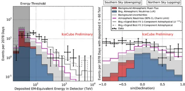
Till now the IceCube detector was the only experiment capable to observe astrophys-ical neutrinos in two independent samples. The first one was an excess of high-energy events over the atmospheric background, detected between May 2010 and May 2013 [31]. The measurement had a statistical significance larger than 6 standard deviations with respect to the only-background hypothesis. The neutrino events were selected with the requirement that the interaction vertex was contained inside the instrumented volume of the detector. This first set of events was defined High Energy Starting Events (HESE). In Fig.1.8 the energy distribution and their sin(declination) is shown. The poor angular resolution does not allow to accurately locate in the sky the source of these neutrino signals. The second data sample was still an excess of diffuse flux of astrophysical neu-trinos. The selection procedure was carried out selecting CC upgoing muon neutrino events [32]. In this sample ∼500,000 muon neutrino candidates were selected with a
Figure 1.8: left: deposited energy, right: arrival direction in IceCube detector of the observed HESE events, compared with predictions (red atmospheric muons and blue the atmospheric neutrinos). The sample refer to 6 years of data. Figure taken from [31].
negligible contamination from atmospheric events. Also for this sample, the significance of the observation respect to the pure background hypothesis was at 6.7 𝜎. The real breakthrough event for neutrino astronomy occurred in September 2017, when IceCube detected a muon-like event induced by a ∼300 TeV neutrino, causing an alert for the searches of 𝛾-ray counterparts. The Fermi-LAT satellite and the MAGIC gamma ray telescope reported a coincidence with neutrino direction of a known 𝛾-ray source, the active galaxy TXS 0506+056 (object classified as a blazar). Neutrino correlation with the registered activity of TXS 0506+056 was classified as statistically significant at the level of 3 𝜎 [33].
Figure 1.9: left: event display of the high-energy neutrino detected by IceCube col-laboration; right: spatial coincidence with the neutrino direction found from FERMI-LAT and MAGIC. Figures taken from [33].
1.3.5 Gravitational wave in the multi-messenger scenario
With the first detection of Gravitational Wave (GW) by the Ligo collaboration in September 2015 [34], a new window on the Universe was opened. Since that moment, lots of other GWs have been detected, but probably the most important one was de-tected in August 2017 by the VIRGO/Ligo collaboration [35]. The first coincidence signal of a GW and its electromagnetic counterpart was announced on 2017 October 16. The astrophysical event, at the origin of the GW, was the coalescence of two neutron stars ∼40 Mpc away from the Earth. From the study of the electromagnetic follow-up in the following days the signatures of synthesised materials, like gold and platinum, was revealed, resolving a long lasting mystery on the nature of the heaviest elements of the periodic table. Also the neutrino signal counterpart was searched by IceCube, ANTARES and Pierre Auger Observatory collaborations but no statistically significant excess was found [36]. After this event, several joint analyses have been conducted by the ANTARES collaboration, together with IceCube and other cosmic ray and 𝛾-ray experiments, considering five events (GW150914, GW151226, LVT 151012, GW170104,
and GW170817), producing no statistical evidence of neutrino involvement [37]. The multi-messenger observations conducted till now, considering both the neutrino-𝛾 and the GW-𝛾 coincidences have replied to important unanswered questions in astrophysics and in particle physics. The possibility in the future, with the advent of the second gen-eration neutrino telescopes, of the detection of a coincidence between GWs and neutrinos would shine a unique light on source properties. Main candidates for a possible coin-cidence are GRBs from core-collapse supernova and binary coalescence of at least one non black-hole object [38]. Furthermore the possible coincident detection can put severe constraints on neutrino mass ordering, and, in the most optimistic scenario, even on the absolute mass of the neutrino itself, thanks to the measurement of the difference between the arrival time of GW and of the incoherent neutrino wave packet. Just to mention, lots of efforts are spent, not only on the experimental site trying to detect these coincidence signals, but also under the theoretical point of view. Several papers, for example, studied the modification of neutrino oscillation when interacts with static gravitational fields. A recent study tries to infer what could be the impact, on astrophysical neutrino mixing, of the interaction with a time dependent gravitational field, as that produced by a GW [39].
Neutrino telescopes and KM3NeT
The idea of a telescope based on the detection of secondary particles produced in neutrino interactions was suggested by Markov and Zheleznykh in 1960 [40]. The ne-cessity of big instrumented volume detectors, due to the small neutrino cross section (𝜎 ∼ 10−38 𝐸
𝜈/𝐺𝑒𝑉), was solved exploiting large and transparent medium given by
nature. This type of detectors registers the Cherenkov light, induced along the path of charged secondary particles, with a large array of photosensitive devices. Using the arrival time of the Cherenkov photons and the position of the photosensors, the direc-tion and energy of the incoming neutrino, as well as other parameters of the neutrino interaction, can be reconstructed.
In the mid-70s the DUMAND collaboration started a pioneering project to deploy a neutrino telescope offshore Hawaii Island [41]. Unfortunately, the technology was not yet mature and the tentative was abandoned. This marked the starting point of a series of other projects: AMANDA at the South Pole [42], which was the precursor of the present large detector IceCube [43]; Baikal, under the water of the lake Baikale, at present expanding towards a km3 structure, named GVD [44]. In the Mediterranean Sea, the
ANTARES experiment [45], located offshore the French southern coasts, is the precursor of the future KM3NeT/ARCA and ORCA detectors that will reach a km3 instrumented
principle, and the main difference consists in the photocathode area density, optimised for the targeted physics goal, which determines neutrino energy threshold. The overall structure of this section and partly also the content is inspired by PhD theses [46–48].
2.1 Detection principle
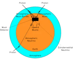
Figure 2.1: Illustration of the possible origin of events and background inside the telescope.
The detection principle in an underwater neutrino telescope is the collection of optical photons, induced along the path of the secondary particles generated in the interaction of neutrinos with the rock under the telescope or with water surrounding it. Depend-ing on the flavour of neutrinos and on the interaction channel, charged (CC) or neutral (NC), different final states are possible. However high-energy muons produced in 𝜈𝜇
charged current interactions represent the golden channel for the identification of neu-trino sources, since they are highly penetrating particles (range in water for 1 TeV muon is several kilometres) and their direction can be reconstructed with high accuracy. Elec-tron neutrinos can be identified through the detection of the particle showers initiated by the charged lepton. Theoretical expectations on neutrino fluxes, see Fig.1.7, and neutrino cross sections suggest that a detection area of the order of 1 km2 is necessary
in order to have a rate of some events/year. These detectors must be shielded from the intense flux of atmospheric muons, originated in the upper parts of the atmosphere over
the detector. At Earth level, the atmospheric muon flux is about 1011 times larger than
the one of atmospheric neutrinos. For this reason the detector must be placed under thousands of metres of water or ice. Even at such depths, the atmospheric muon flux is six orders of magnitude larger than that of muons induced by atmospheric neutrinos, and is able to generate in the telescope a top-bottom signal: these are called downgoing
events. In order to reject part of this overwhelming background, a geometrical selection
of the events upward going is applied onto the tracks, after their reconstruction, because only neutrinos can cross the Earth producing charged particles coming from below. In this case the telescope registers a bottom-top signal, producing what are called upgoing
events. Muons are absorbed within a path of about 50 km of water, and they are not
able to traverse the entire Earth diameter (∼13 000km).
Even upgoing events suffer background due to misreconstructed downgoing events.
2.1.1 Cherenkov radiation
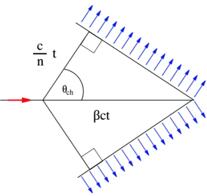
The Cherenkov radiation is generated by the passage of charged particles through a dielectric medium with refractive index n, with a velocity greater than the speed of light in that medium (𝑐/𝑛). The charged particles polarise the molecules along the trajectory, and only when the electrons come back to their ground state, they emit a coherent radiation. The light is emitted at a characteristic angle 𝜃𝑐ℎ, as depicted in Fig.2.2. The opening angle depends on the particle velocity 𝛽 = 𝑣/𝑐 and on the refractive index n of the medium:
𝑐𝑜𝑠(𝜃𝑐ℎ) = 𝑐/𝑛 𝛽𝑐 =
1
𝛽𝑛 (2.1)
In water n ≈ 1.35 and the Cherenkov angle for relativistic particles (𝛽 ≈ 1) is 𝜃𝑐ℎ ≈ 42°.
The number of emitted photons per path length dl and wavelength interval d𝜆 is given by the Frank-Tamm formula:
𝑑2𝑁
= 2𝜋𝛼𝑧
2
Figure 2.2: The outlined angle is 𝜃𝑐ℎ. The red arrow represents the propagation
direction of the charged particle. The blue arrows show the propagating wave front of the produced light.
where 𝛼 is the fine-structure constant. In the wavelength range from 300 nm to 600 nm, in which the water is transparent, the number of photons per particle path length is approximately:
𝑑𝑁
𝑑𝑙 ∣𝑤𝑎𝑡𝑒𝑟 = 340 𝑐𝑚
−1 (2.3)
Cherenkov radiation however occurs only for 𝛽 > 1/𝑛. Therefore the energy threshold E𝑡ℎ, for a particle with rest mass m0 is:
𝐸𝑡ℎ = 𝑚0
√1 − 1/𝑛2 (2.4)
In water this corresponds to a threshold kinetic energy (T𝑡ℎ=E𝑡ℎ-m0) T𝑒𝑡ℎ ≈ 0.25 MeV
for electrons, T𝜇
𝑡ℎ≈ 53 MeV for muons and T 𝑝
2.1.2 Light propagation
Once the light is produced, other physical effects influence the signature of Cherenkov light: absorption and scattering in water. While the first one affects the number of pho-tons, the latter influences the direction and arrival time of photons on the photosensors. In order to describe properly these two effects, two key parameters must be introduced, the absorption length 𝜆𝑎𝑏𝑠(𝜆) and the scattering length, 𝜆𝑠(𝜆). The absorption
param-eter corresponds to the total photon path length after which the survival probability is reduced by 1/e. Optically pure seawater shows the highest transparency for photon wavelength of about ∼ 400 nm, where typical values of 𝜆𝑎𝑏𝑠 ≈ 60m are reached. When
one considers scattering, 𝜆𝑠 and the angular distribution of the momentum of the
outgo-ing particles must be taken into account, because both contribute to the definition of an effective scattering length. The scattering typically occurs on water molecules (‘Rayleigh scattering’) and on larger particulates (‘Mie scattering’), resulting in a small total scat-tering angle over the detectable wavelength range. The effective scatscat-tering length is defined as:
𝜆𝑒𝑓𝑓𝑠 = 𝜆𝑠/[1 − ⟨𝑐𝑜𝑠(𝜃𝑠)⟩] (2.5)
where ⟨𝑐𝑜𝑠(𝜃𝑠)⟩ is the average scattering angle. In seawater typical values of 𝜆𝑠 ≈ 55 m
and 𝜆𝑒𝑓𝑓
𝑠 ≈ 265 m have been measured for photon wavelength of 470 nm.
2.2 KM3NeT detector
KM3NeT1 is a research infrastructure housing the next generation neutrino
tele-scopes. Once completed, it will host a network of Cherenkov detectors, reaching, in its final configuration, an instrumented volume of several cubic kilometres of sea water. It is located at the bottom of the Mediterranean Sea, and its design was driven by the
rience gathered with the first generation neutrino telescopes, especially ANTARES. This detector in fact has demonstrated the feasibility of the Cherenkov technique in deep sea for neutrino detection. KM3NeT comprises two different instrumented regions, placed in separate locations: KM3NeT/ARCA2, off-shore Sicily coasts, whose goal is the search
of neutrinos generated from astrophysical sources, and KM3NeT/ORCA3, off-shore the
French Southern coasts that will study neutrino properties exploiting atmospheric neu-trinos generated in the Earth’s atmosphere. Both detectors will use the same technology and neutrino detection principle, namely a 3D array of photosensors capable to detect Cherenkov light produced along the path of relativistic particles emerging from neutrino interactions. The main difference is the density of photosensors, which is optimised for the study of neutrinos in the few-GeV (ORCA) and TeV-PeV energy range (ARCA), respectively. The facility will also house instrumentation for Earth and Sea sciences for long-term and on-line monitoring of the deep sea environment and the sea bottom at depth of several kilometres [49]. The following sections were inspired by [46].
2.2.1 Installation sites
The Mediterranean Sea offers optimal conditions to host an underwater neutrino tele-scope. Several sites were studied and characterised, and the deploy feasibility evaluated through different criteria such as: distance from the coast, sufficient depth in order to reduce the atmospheric muon background, good optical properties of the water, low level of bio-luminescence, low rates of sedimentation and stable low sea current velocities. The three locations selected are shown in Fig.2.3.
KM3NeT/ORCA Deployed at the KM3NeT-Fr installation site, about 40 km off-shore Toulon, France, the ORCA neutrino detector will achieve the angular and energy
2ARCA stands for Astroparticle Research with Cosmics in the Abyss 3ORCA stands for Oscillation Research with Cosmics in the Abyss
Figure 2.3: Map of the location of the 3 sites for the construction of the KM3NeT neutrino telescope in the Mediterranean Sea. KM3NeT-Gr is located off the coast of Pylos. At present, it is used only for validation and qualification. Taken from [50]. resolution required for resolving the neutrino mass hierarchy. The sensor modules are arranged on vertical detection units with a height of about 200 m and in the dense configuration required for detection of neutrinos with energies as low as about a GeV. During February 2020 sea campaign, 7-strings configuration with a horizontal spacing of about 20 m has been achieved. In the next construction phase (KM3NeT 2.0), full ORCA will comprise a building block of 115 detection units.
KM3NeT/ARCA instead is being installed at the KM3NeT-It site, about 100 kilo-metres off-shore the town of Portopalo di Capo Passero in Sicily, Italy. The detection units of the ARCA telescope will be anchored at a depth of about 3500 m. In its fi-nal configuration the ARCA telescope will consist of two building blocks of 115 vertical
detection units each, resulting in an instrumented volume of about 1 cubic kilometre – slightly larger than IceCube neutrino telescope. The construction of ARCA, at the end of Phase-1, will contain 24 detection units, reaching a volume of about 0.1 cubic kilometre.
Figure 2.4: Sky coverage of KM3NeT detectors. Some known astrophysical objects are marked. Figure taken from [51].
Both sites are in the Northern hemisphere at a latitude between 36° and 43° North, allowing to observe upgoing events coming from most of the sky. Looking at the KM3NeT sky coverage, reported in Fig.2.4, most of the Galactic plane, including the Galactic centre, is visible. This is an advantage considering the sources hosted in the centre of our Galaxy, and KM3NeT is able to complement the field of view of IceCube telescope, located at the South Pole.
2.2.2 Digital Optical Module (DOM)
The ‘Digital Optical Module’ (DOM) developed by the KM3NeT collaboration is the active part of the neutrino telescope and consists of a transparent 17-inch diameter pressure-resistant glass sphere, housing 31 3-inch PMTs, their associated readout
elec-Figure 2.5: Photograph of the Digital Optical Module (DOM) of KM3NeT complete (left) and in assembly phase (right). Taken from [46].
tronics and additional sensors, as shown in Fig.2.5. The task of the DOM is to register the time of arrival of the Cherenkov light generated in the sea water inside or close to the detector; the modules also measure their geometrical position at the arrival time of the light. The PMTs have a standard bialkali photo-cathode with quantum efficiency of 28% at 404 nm and 20% at 470 nm. Moreover this multi-PMT configuration offers some advantages compared to more traditional designs based on large-area PMTs, such as: (i) maximisation of the photocatode area in a single sphere; (ii) small PMTs are less sensitive to Earth magnetic field, not requiring metal shielding; (iii) segmentation of the detection area, improving the discrimination between single-photon and multi-photon hits.
The PMTs are arranged in 5 rings of tubes at zenith angles of 50°, 65°, 115°, 130° and 147°, respectively. In each ring there are 6 PMTs and a single PMT is placed at the bottom, with a zenith angle of 180°: therefore 19 PMTs are placed in the lower hemisphere and 12 PMTs in the upper hemisphere of the DOM. Each PMT is surrounded by a reflector ring in order to increase the photon collection efficiency (20-40% depending on photon incident angle), and optical gel fills the cavity between PMT and glass sphere in order to assure optical contact. An active base is also attached to the PMT allowing to
Figure 2.6: Exploded view of the KM3NeT DOM.Taken from [52].
control from shore the high-voltage power supply (∼ 1000 V), and threshold settings for each tube. This board has been miniaturized in order to fit in the limited space available inside the glass sphere. When a photon hits the photomultiplier tube, a small electrical pulse is created. The pulse is then amplified and transformed into a square wave pulse, by the time-over-threshold (ToT) technique (the amount of light is transformed to an amount of charge which is translated to the length of the square wave pulse), and sent to the Field Programmable Gate Array (FPGA), hosted on the Central Logic Board (CLB), where its arrival time and its pulse length is registered and stored for a later transfer to shore. The internal structure of the DOM has been carefully designed to efficiently dissipate the heat generated from the electronics using a mushroom shaped
aluminium structure that transfers it to the sea via the glass sphere, see Fig.2.6. The DOM also contains other sensors used for calibration purposes: a compass to know the pointing direction of each photomultipliers; accelerometres to know tilt, pitch and yaw of the module; a piezo-acoustic sensor allows the determination of the position of the DOM exploiting a sonar technique. All these measurements are important as the DOMs move under the influence of sea currents. In ANTARES, this calibration devices can locate the photosensors with an uncertainty of less than 10 cm.
2.2.3 Detection Unit (DU) and detector layout
Figure 2.7: Schematic outline of a KM3NeT/ARCA building block. Taken from [53] A collection of 18 DOMs connected to an electro-optical cable and arranged along a vertical structure with two ropes is called Detection Unit or DU (or string) for short. A detection unit has an anchor, which keeps it firmly connected to the seabed. Even though the DU design minimises drag and by itself is buoyant, additional buoyancy is introduced at the top of the string to reduce the horizontal displacement of the top in

![Figure 2.6: Exploded view of the KM3NeT DOM.Taken from [52].](https://thumb-eu.123doks.com/thumbv2/123dokorg/7385414.96827/49.892.278.612.158.641/figure-exploded-view-km-net-dom-taken.webp)
![Figure 2.7: Schematic outline of a KM3NeT/ARCA building block. Taken from [53] A collection of 18 DOMs connected to an electro-optical cable and arranged along a vertical structure with two ropes is called Detection Unit or DU (or string) for short](https://thumb-eu.123doks.com/thumbv2/123dokorg/7385414.96827/50.892.166.734.503.802/schematic-building-collection-connected-arranged-vertical-structure-detection.webp)

