AGE-SPECIFIC PROBABILITY OF CHILDBIRTH. SMOOTHING
VIA BAYESIAN NONPARAMETRIC MIXTURE OF ROUNDED
KERNELS
Antonio Canale1
Dipartimento di Scienze Economico-Sociali e Matematico-Statistiche, Universit`a di Torino, Torino, Italia e Collegio Carlo Alberto, Moncalieri, Italia
Bruno Scarpa
Dipartimento di Scienze Statistiche, Universit`a di Padova, Padova, Italia.
1. Introduction
Milan is the main industrial, commercial and financial center in Italy by hosting the headquarters of the largest national companies and banks. Its municipality is the second largest municipality in Italy with almost 1.3 millions of residents (ISTAT, 2013) while its urban area is the largest in Italy. It is also a multiethnic city, being the destination of, national and international, immigration with almost the 20% of the total resident population made of foreign-born residents.
In such a large and multicentric city, the different areas may be characterized by different sub-population with different economical status or social behavior. Clearly, in such a context, policy makers are interested in understanding socio-demographical and economical differences among areas, in order to choose correct decisions. For example, Milan is divided in nine areas (zone di decentramento) having partial political autonomy, which may require an accurate knowledge of specific population social needs.
In this paper we concentrate on estimating differences in fertility among the nine areas of Milan. The knowledge of age-specific fertility indicators in different areas of large urban centers is extremely useful in order to make informed political decision. For example, it may be useful to decide where to build a new nursery-school, where to increase obstetrics departments in hospitals, or which kind of services can be offered to mothers and families.
We use the opendata made available by the Municipality of Milan, counting all the childbirths in Milan in 2011 divided by areas and mother’s age and we estimate the different age-specific probabilities of childbirths.
Even in a big cities, the simple, and quite used for large populations, empirical estimator of fertility curves, based on the counting of childbirths in a given year
by area and mother’s age is affected by the typical variability related to random noise. Therefore a statistical model is needed to describe fertility in detail and discuss the differences.
A large number of models have been proposed in demographical literature to describe fertility curves of large populations (see for example Mazzuco and Scarpa, 2013, for a recent review); however, much less attention has been given to models for local fertility curves, where we expect a wider variety of patterns than for the country level. In large populations, fertility curves for developed countries are moving from the classical right-skewed shape to a symmetric one due to the fact that women with higher educational level tend to delay childbirth. Also, is some developed countries, fertility curves exhibit an almost bimodal shape, due to a hump appearing around 20 years; this could be related to the presence of different subpopulations. For example US, UK and Ireland fertility curves show this pattern due to higher levels of young women pregnancy in lower classes.
Although for city level we do not have specific studies to describe fertility, in some areas of Milan we may expect to observe the symmetric pattern, particu-larly, in those areas where most of the resident women have middle-high educa-tional level. On the other side in some other peripheral areas we may observe the bimodal behavior, given the presence of a subpopulations of foreigners, with different average ages at childbirth. Moreover, in other areas of a city as Milan we may also expect different patterns, such as, for example, a left-skewed curve, related to a generalized very long delay in childbirth.
Given this variety of possible patterns, a nonparametric approach seems ap-propriate to both smooth the random noise affecting the curves, and to account for different patterns. Skewness and multimodality can be modelled via mixture models. It is known, for example, that a mixture of Gaussians kernels can consis-tently estimate the shape of almost any continuous distribution. As discussed by many authors (Chandola et al., 1999; Ortega Osona and Kohler, 2000; Peristera and Kostaki, 2007; Schmertmann, 2003), mixture models are clearly appropriate when two or more populations with different age-specific fertility rates are present. However, the problem of choosing the number of mixture component remains elu-sive in most applications.
In the following we use a Bayesian nonparametric mixture model to fit age-specific probabilities of childbirths. A Bayesian nonparametric mixture allows us to obtain a dramatic degree of flexibility as it is able to fit a potential infinite number of mixture components. The price to pay in terms of model complexity is however very small, given the recent contributions in Markov Chain Montecarlo (MCMC) sampling procedures. Furthermore, since the open data on childbirth are rounded, in the sense that we only have the mother’s age in years, we propose a model which account for this discrete scale in which data are available. In the next section we present the model and, in the following one, we show and discuss some results for the Milan data.
2. The model
Let y be the age of the mother at childbirth and assume that we want to model the probability distribution p(y). In fact, even if age is ideally continuous, it is typically rounded to the lower integer when recorded, and so are the opendata available for Milan. Hence p(y) is a probability mass function defined on the positive integers.
We propose to estimate p(y) with a Bayesian nonparametric approach. Bayesian nonparametrics is a relatively young area of research which has recently received abundant attention in the statistical literature. The considerable degree of flexi-bility it ensures, if compared to standard parametric alternatives, and the recent development of new and efficient computational tools, have pushed its concrete use in a number of complex real world problems. Some of the most successful models in Bayesian nonparametrics are Dirichlet process (DP) mixture models. A DP mixture model for probability mass function estimation assumes
p(y) =
∫
K(y; θ)dP (θ), P ∼ DP (α, P0),
where K(·; θ) is a discrete kernel parametrized by a parameter vector θ and P is a random probability mixing measure which has a DP prior (Ferguson, 1973, 1974). The DP is parametrized by α, a scalar precision parameter, and a base measure
P0. The DP can be seen as a probability measure over the space of probability measures. DP mixtures are widely used in continuous density estimation and in particular using Gaussian kernel in place of K(·; θ) (Lo, 1984; Escobar and West, 1995). This DP mixture of Gaussians is computationally convenient and has nice theoretical properties. Marginalizing out P , from equation above, one can obtain
p(y) = ∞ ∑ h=1 πhK(y; θh), θh iid ∼ P0, π ={πh} ∼ Stick(α)
where Stick(α) denotes the stick-breaking process of Sethuraman (1994). This stick-breaking representation shows that mixture models can be useful for estimate data made of different sub-populations.
Although Bayesian nonparametric mixture models for continuous data are well developed, there is a limited literature on related approaches for discrete data. Following Canale and Dunson (2011), we assume that y = h(y∗), where h(·) is a rounding function defined so that h(y∗) = j if y∗∈ (j − 1, j], for j = 0, 1, . . .. This assumption, introduced in a more general way, for computational and theoretical convenience by Canale and Dunson (2011), matches the data generating process that we are considering. Under this setting the probability mass function p of y is p = g(f ), where g(·) is the rounding function having the simple form
p(j) = g(f )[j] =
∫ j j−1
f (y∗)dy∗ j∈ N.
prior for the distribution of the latent y∗. We assume
y = h(y∗), y∗∼ f∗,
f∗(y) =∑∞h=1πhfN(y∗; µh, σ2h) (1)
with π ∼ Stick(α), (µh, σ2h) ∼ P0 and fN being the gaussian distribution µ∈ ℜ
and σ2∈ ℜ+.
To complete the prior specification we assume α ∼ Ga(1/2, 1/2) as Escobar and West (1995) and P0to be a diffuse normal-inverse-gamma. This choice reflects low prior information on the values of the parameters of each mixture component, which is a common practical choice in Bayesian nonparametrics.
To fit the model to real data we rely on the efficient Gibbs sampling algorithm proposed by Canale and Dunson (2011), as implemented in the R package rmp (Canale and Lunardon, 2013).
3. Fertility in Milan municipality
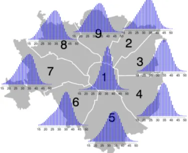
Data on births on the municipality of Milan divided in areas are available on the website dati.comune.milano.it for the years 2003-2011 divided by neigh-borhoods and areas. We consider here the more recent data and the subdivision by areas. The nine areas of Milan include the following neighborhoods: area 1 -historical center; area 2 - central station, Gorla, Turro, Greco, Crescenzago; area 3 - Citt`a Studi, Lambrate, Venezia; area 4 - Vittoria, Forlanini; area 5 - Vigentino, Chiaravalle, Gratosoglio; area 6 - Barona, Lorenteggio; area 7 - Baggio, De An-geli, San Siro; area 8 - Fiera, Gallaratese, San Leonardo, Quarto Oggiaro; area 9 - Garibaldi station, Niguarda. A map with the 9 areas is reported in Figure 1.
We run the Gibbs sampler for 6,000 iterations, discarding the first 1,000 as a burn-in. The remaining 5,000 samples were used to calculate the posterior mean of the probability mass function for j = 15, . . . , 50. As posterior estimate, we consider the mean probability mass functions in the nine areas, reported in Figure 1 over the maps of Milan.
From this figure it is clear that the distributions of the different areas have different shapes. For example, area 1, 3, and 5 are almost symmetric with, in area 3, only mild left skewness. These probability mass functions clearly show a delay in childbirth, with respect to classical curves, but suggest also the presence of a common fertility behaviour inside these areas. Other areas, instead, present a small hump around 20-25 years. In area 4 and 6 this is clearly evident, while in area 8 and 9 this is only partially noticeable. The former areas are likely to have at least two subpopulations, with the smaller consisting in women anticipating the childbirth. Most of the estimated probability mass functions exhibit moderate skewness to the left, sign of a general trend of the majority of women in the area to postpone the age at childbirth, but also indicator of the presence of subgroups that anticipate it.
Our procedure allows for borrowing of information across the age of childbirth. Indeed, from Figure 2, which compares for each area our estimates along with the empirical estimates, it is clear that the mean of the posterior probability mass function is smoother than the empirical estimate, which has an erratic behaviour
Figure 1 – Posterior mean probability mass function for the age of the mother at
106 A ntonio Canale and Bruno Sc arp 0.00 0.04 0.08 0.12 Zone 1 age
age−specific probability of childbir
ths 15 18 21 24 27 30 33 36 39 42 45 48 51 empirical gaussian−mix 0.00 0.04 0.08 0.12 Zone 2 age
age−specific probability of childbir
ths 15 18 21 24 27 30 33 36 39 42 45 48 51 empirical gaussian−mix 0.00 0.04 0.08 0.12 Zone 3 age
age−specific probability of childbir
ths 15 18 21 24 27 30 33 36 39 42 45 48 51 empirical gaussian−mix 0.00 0.04 0.08 0.12 Zone 4 age
age−specific probability of childbir
ths 15 18 21 24 27 30 33 36 39 42 45 48 51 empirical gaussian−mix 0.00 0.04 0.08 0.12 Zone 5 age
age−specific probability of childbir
ths 15 18 21 24 27 30 33 36 39 42 45 48 51 empirical gaussian−mix 0.00 0.04 0.08 0.12 Zone 6 age
age−specific probability of childbir
ths 15 18 21 24 27 30 33 36 39 42 45 48 51 empirical gaussian−mix 0.00 0.04 0.08 0.12 Zone 7 age
age−specific probability of childbir
ths 15 18 21 24 27 30 33 36 39 42 45 48 51 empirical gaussian−mix 0.00 0.04 0.08 0.12 Zone 8 age
age−specific probability of childbir
ths 15 18 21 24 27 30 33 36 39 42 45 48 51 empirical gaussian−mix 0.00 0.04 0.08 0.12 Zone 9 age
age−specific probability of childbir
ths
15 18 21 24 27 30 33 36 39 42 45 48 51 empirical
gaussian−mix
Figure 2 – Posterior mean probability mass function (blue bars) with pointwise 95% credible bands (dashed blue lines) and empirical
ecific pr ob ability of childbirth 107 TABLE 1
Posterior summaries in the nine different administratives areas of the municipality of Milan. Posterior predictive mean and variance, posterior predictive probability of young and old age at childbirth, averege number of occupied mixture components.
E(yn+1|ˆp) Var(yn+1|ˆp) pr(yn+1≤ 19|ˆp) pr(yn+1≤ 25|ˆp) pr(yn+1≥ 40|ˆp) # of clusters
Area 1 34.86 4.65 0.00 0.01 0.14 4.94 Area 2 32.25 5.91 0.00 0.08 0.10 5.27 Area 3 33.35 5.81 0.00 0.06 0.14 4.81 Area 4 32.60 5.80 0.00 0.08 0.10 4.17 Area 5 32.67 5.99 0.01 0.07 0.12 3.76 Area 6 32.98 5.97 0.01 0.08 0.12 3.62 Area 7 32.50 5.98 0.01 0.08 0.11 4.98 Area 8 32.11 6.07 0.01 0.09 0.10 4.33 Area 9 31.96 5.94 0.00 0.09 0.10 4.06
20 30 40 50 60 0.00 0.02 0.04 0.06 age
age−specific probability of childbir
th
Figure 3 – Posterior mean probability mass function of area 6 with the two principal
mixture components.
by chance. However, our procedure is also able to catch the shape of each prob-ability mass function, which, as we already discuss, is quite different one from another. Pointwise 95% credible bands are also reported to show posterior vari-ability. These are calculated taking the empirical quantiles of each MCMC chain after burn-in. The posterior variability is similar in each area with wider credible intervals for the central ages and thinner intervals for high and low age of the mother.
In Table 1, we report some posterior mean estimates of some interesting quan-tities. The posterior predictive mean represent the estimated average in each area. This is generally high, over 31 years, but there are considerable differences between different areas. The higher mean is recorded in the central area 1 and is 34.86 while the lower is recorded in area 9, being almost 32 years. The probability of deliver in young age is very low for every area, and again the “oldest” mothers are in area 1 (pr(y ≤ 25) = 0.01 and pr(y ≥ 40) = 0.14) and the “youngest” in area 9 (pr(y≤ 25) = 0.09 and pr(y ≥ 40) = 0.1).
Because of the likely presence of sub-populations in some areas, an interesting posterior quantity is given by the average number of occupied clusters in the mixtures. This is reported in the last column of Table 1. At a first glance it may surprise to see that the unimodal and symmetric probability of area 1, has almost 5 occupied clusters on average; however, the posterior variability associated to this, is very high suggesting that mixture is used simply to better fit the data without any claim of interpretation. On the other side, for example, area 6 has an average number of occupied clusters equal to 3.62; as interpretation this suggests the cohabitation in the area of a small number (two or three) of groups of women
with different behaviours in terms of fertility. This is also indicated by the hump on the left (see Figure 1 and 2). To better perceive the presence of the two possible subpopulations, Figure 3 shows the posterior density along with the two most populated clusters.
To conclude, we want to notice that a simpler parametric model could be used to estimate the probability of age at childbirth in each single area, for the symmetric shapes the choice of the parametric model being quite easy, and for the skew and almost bimodal one being more tricky. However, the choice of a nonparametric flexible approach is preferable in absence of prior information on the shape of the distributions and is very flexible to catch all the shapes of the different areas.
4. Discussion
Open data are a formidable way to empower citizens, help small businesses, create value in positive and constructive ways. The Municipality of Milan initiative to diffuse administrative data and start collaborative projects is certainly the beginning of a fascinating and challenging path to improve education and to help government and policy makers to better exploit the available information.
We presented a statistical model to describe fertility curves by areas. The pro-posed model describes the probability of childbirth and deals with the different shapes observed in the nine areas of the city of Milan. The nonparametric charac-teristic of our model allows for smoothing the random variability due to the small size of the data for some age and area, but its specific formulation, based on almost certainly finite mixture of gaussian kernels, enables for a clear interpretation of the results.
Interesting results describing the variability of fertility between the nine Mi-lan areas are sketched and discussed, leading to hints for further investigation of demographical and socio-economical interpretations.
References
A. Canale, D. B. Dunson (2011). Bayesian kernel mixtures for counts. Journal of the American Statistical Association, 106, no. 496, pp. 1528–1539.
A. Canale, N. Lunardon (2013). R package rmp: Rounded Mixture Package. T. Chandola, D. Coleman, R. W. Hiorns (1999). Recent European fertility
patterns: Fitting curves to ’distorted’ distributions. Population Studies, 53, pp.
317–329.
M. D. Escobar, M. West (1995). Bayesian density estimation and inference
using mixtures. Journal of the American Statistical Association, 90, pp. 577–588.
T. S. Ferguson (1973). A Bayesian analysis of some nonparametric problems. The Annals of Statistics, 1, pp. 209–230.
T. S. Ferguson (1974). Prior distributions on spaces of probability measures. The Annals of Statistics, 2, pp. 615–629.
ISTAT (2013). Popolazione residente al maggio 2013. www.demo.istat.it. A. Y. Lo (1984). On a class of Bayesian nonparametric estimates: I. Density
estimates. The Annals of Statistics, 12, pp. 351–357.
S. Mazzuco, B. Scarpa (2013). Fitting age-specific fertility rates by a
flexi-ble generalized skew-normal probability density function. Journal of the Royal
Statistical Society: Series A.
J. A. Ortega Osona, H.-P. Kohler (2000). A comment on “Recent European
fertility patterns: fitting curves to ’distorted’ distributions”, by T. Chandola, D. A. Coleman and R. W. Hiorns. Population Studies, 54, pp. 347–349.
P. Peristera, A. Kostaki (2007). Modelling fertility in modern populations. Demographic Research, 16, pp. 141–194.
C. P. Schmertmann (2003). A system of model fertility schedules with graphically
intuitive parameters. Demographic Research, 9, pp. 82–110.
J. Sethuraman (1994). A constructive definition of Dirichlet priors. Statistica Sinica, 4, pp. 639–650.
Summary
The municipality of Milan is one of the most important areas in Italy being the center of many economic activities and the destination of strong national and international immigration. In this context, policy makers are interested in understanding socio-demographical and economical differences among the different urban areas. In this paper we concentrate in estimating differences in fertility among the nine areas of Milan. The knowledge of age-specific fertility indicators, indeed, is extremely useful in order to de-cide where to build a new nursery-school, where to increase obstetrics departments in hospitals, or which kind of services can be offered to families. To estimate the age-specific probabilities of childbirths in the municipality of Milan, we use opendata on the births residents in Milan in 2011. It has recently been observed that the patterns of fertility of developed countries show a deviation from the classic right-skewed shape due to the fact that women tend to have children later. Also, when a large component of immigrants is present, the age-specific fertility rate exhibits an almost bimodal shape, the curve shows a little hump between 20 and 25 years of the woman, presumably due to the pres-ence of subpopulations. To deal with this phenomena and to compare fertility between the nine urban areas of the municipality of Milan, we apply a Bayesian nonparametric mixture model which can account for skewness and multimodality and we estimate the age-specific probability of childbirth.