Alma Mater Studiorum – Università di Bologna
DOTTORATO DI RICERCA IN
Ingegneria Ambientale, Civile e dei Materiali
Ciclo XXVII
Settore Concorsuale di afferenza: 08 A2 Settore Scientifico disciplinare: ING/IND 30
TITOLO TESI
Valorisation of organic waste: new developments from proton nuclear
magnetic resonance characterization
Presentata da: Marianna Vannini
Coordinatore Dottorato
Relatore
Alberto Lamberti
Villiam Bortolotti
i
Abstract
The last half-century has seen a continuing population and consumption growth, increasing the competition for land, water and energy. The solution can be found in the new sustainability theories, such as the industrial symbiosis and the zero waste objective. Reducing, reusing and recycling are challenges that the whole world have to consider. This is especially important for organic waste, whose reusing gives interesting results in terms of energy release. Before reusing, organic waste needs a deeper characterization. The non-destructive and non-invasive features of both Nuclear Magnetic Resonance (NMR) relaxometry and imaging (MRI) make them optimal candidates to reach such characterization. In this research, NMR techniques demonstrated to be innovative technologies, but an important work on the hardware and software of the NMR LAGIRN laboratory was initially done, creating new experimental procedures to analyse organic waste samples. The first results came from soil-organic matter interactions. Remediated soils properties were described in function of the organic carbon content, proving the importance of limiting the addition of further organic matter to not inhibit soil processes as nutrients transport. Moreover NMR relaxation times and the signal amplitude of a compost sample, over time, showed that the organic matter degradation of compost is a complex process that involves a number of degradation kinetics, as a function of the mix of waste. Local degradation processes were studied with enhanced quantitative relaxation technique that combines NMR and MRI. The development of this research has finally led to the study of waste before it becomes waste. Since a lot of food is lost when it is still edible, new NMR experiments studied the efficiency of conservation and valorisation processes: apple dehydration, meat preservation and bio-oils production. All these results proved the readiness of NMR for quality controls on a huge kind of organic residues and waste.
iii
Nomenclature
1H NMR = Proton Nuclear Magnetic Resonance
BET = Brunauer–Emmett–Teller adsorption technique CPMG = Carr-Purcell-Meiboon Gill
FID = Free Induction Decay FOV = Field Of View
FT = Fourier Transform FW = Food Waste IR = Inversion Recovery
LAPSRSE = Logarithmically Aperiodic Saturation Recovery Spin Echo MIP = Mercury Injection Porosimetry
MRI = Magnetic Resonance Imaging MRR = Magnetic Resonance Relaxometry NMR = Nuclear Magnetic Resonance OM = Organic Matter
PSD = Pore Size Distribution
QRT = Quantitative Relaxation Tomography RF = Radiofrequency
SE = Spin Echo
S/N = Signal to Noise ratio SR = Saturation Recovery
TD-NMR = Time-Domain Nuclear Magnetic Resonance TD-MRR = Time-Domain Magnetic Resonance Relaxometry
iv
B0 = static (external magnetic field)
B1 = induced magnetic field
T1 = spin lattice or longitudinal relaxation time
T2 = spin spin or transverse relaxation time
R1 = spin lattice or longitudinal relaxation rate
R2 = spin spin or transverse relaxation rate
ρ = surface relaxivity
S/V = surface to volume ratio φ = porosity
TE = Time of Echo TR = Time of Repetition
v
1
Alma Mater Studiorum – Università di Bologna
Valorisation of organic waste: new developments from proton nuclear
magnetic resonance characterization
1
Abstract i
Nomenclature iii
Chapter 1 9
Introduction 9
1.1 The importance of the characterization, identification and valorisation of waste driving
toward a zero waste society 11
Chapter 2 17
Low-field Nuclear Magnetic Resonance 17
2.1 Introduction to low-field NMR application to industrial processes 18
2.2 Basics of NMR theory 20
2.3 NMR relaxation and Bloch’s equations 24
2.3.1 How to do a NMR experiment: rf pulse sequences 27
2.3.2 T1 measurements 28
2.3.3 Field inhomogeneities and T2 measurements 30
2.3.4 NMR Relaxation in porous media 32
2.3.5 Paramagnetic impurities 37
2.3.6 NMR Relaxation in biological systems 38
2.5 NMR Imaging 40
2.5.1 The principles of images reconstruction 40
2.5.2 K-space 44
2.5.3 Frequency and phase encoding 44
2.5.4 Contrast in MRI 46
2.5.6 Saturation recovery sequence 48
2.5.7 Quantitative Relaxation Tomography (QRT) technique 48
Chapter 3 51
NMR equipment: hardware and software optimization for measurements on organic
waste 51
3.1 New hardware and software releases 53
3.2 Hardware optimization 53
3.2.1 The NMR permanent magnet of the laboratory 53
3.2.2 The dedicated NMR coils for relaxometry: new configurations and updates 55
3.2.3 Signal-to-noise ratio problems 57
3.2.4 An home-made bio-reactor device for NMR measurements 60
3.3 Software optimization 61
3.3.1 The creation of a dedicated NMR sequence: the Logarithmic A-Periodic Saturation Recovery
Spin Echo (LAPSRSE) sequence 62
3.3.2 The LAPSRSE generator software 64
3.3.3 A tool for NMR data pre-inversion processing: the “Field Cycling” software 69
vi
3.3.5 The creation of a tool for NMR data post-inversion processing: the “FiltroDAT” software 72
3.3.6 ARTS for MRI 74
3.3.7 PERFIDI sequences optimization 75
Chapter 4 79
Paper waste for soil recovery: how organic matter influences soil properties 79
4.1 Introduction 81
4.2 Materials and methods 86
4.2.1 Samples and TOC analysis 86
4.2.2 Scanning Electron Microscopy coupled to Energy Dispersive Spectroscopy 87
4.2.3 X-ray Diffraction 87
4.2.4 1H-MRR measurements 88
4.2.5 T1 cut-off determination 89
4.2.6 Relaxivity evaluation 90
4.2.7 N2 adsorption/desorption measurements at -196°C 94
4.3 Results and discussion 94
4.3.1 Samples standard analyses 94
4.3.2 SEM and XRD results 95
4.3.3 N2 adsorption/desorption results 97
4.3.4 1H-MRR results 100
4.4 Conclusions 106
Chapter 5 107
Organic waste for composting: an insight of the biodegradation process 107
5.1 Introduction 109
5.2 Materials and methods 111
5.2.1 Samples 111
5.2.2 Temperature and pH measurements 112
5.2.3 MRR and QRT measurements 113
5.3 Results and discussion 115
5.3.1 Temperature and pH 115
5.3.2 MRR 116
5.3.3 QRT 119
5.4 Conclusions 124
Chapter 6 125
Further developments of the NMR techniques in the organic waste chain 125
6.1 Dehydration of fruit to reduce fruit waste 127
6.1.1 The importance of reducing food waste 127
6.1.2 Apple osmodehyration results 128
6.2 Applications of PERFIDI sequences on meat 130
6.2.1 Meat industry and its impact on food waste 130
6.2.2 PERFIDI sequences for MRI results: validation and proof on meat 131
6.3 Evaluation of bio-oils quality 133
6.3.1 Bio-oil as biomass valorisation products 133
vii 6.4 Summary 136 Conclusions 139 APPENDIX A 143 APPENDIX B 146 APPENDIX C 152 Bibliography 153
9
Chapter 1
Introduction
11
1.1 The importance of the characterization, identification and
valorisation of waste driving toward a zero waste society
Agricultural, food and industrial waste is generated daily in extensive quantities, producing a significant problem in its management and disposal. A widespread feeling of “environment in danger” is increasing in our society year by year, which, however, is not yet crystallized in a general consciousness of cutting waste production in our daily lives. Landfill, incineration and composting are common, mature technologies for waste disposal. However, they entail many problems related to the generation of toxic methane gas and bad odour, high energy consumption and slow reaction kinetics (Arancon et al.; 2013).
Since the development of innovative systems to maximize the recovery of useful materials and/or energy in a sustainable way has become necessary, a new concept, the industrial symbiosis concept, is becoming popular in both scientific and sociological field. Industrial wastes are generated through different industrial processes or energy production utilities as surplus materials. The industrial symbiosis theory defines non-deliberately produced material as by-products or valuable raw materials which can be exploited in other industrial ways.
12
This idea is inspired by the nature cycles, where the concept of waste does not exist (Figure 1.1.a). Industrial symbiosis is the ingenious idea that one company’s waste becomes another’s raw material, leading to enormous carbon, costs and resources savings (Figure 1.1.b).
The percentage and weight of waste components in a solid waste stream are important data for decision-makers. This information is necessary to plan waste reduction and recycling programmes to reach the zero waste objective.
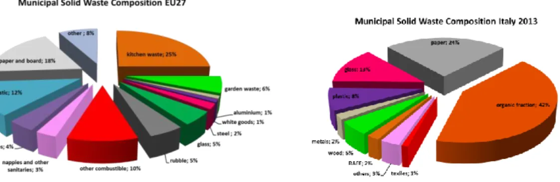
According to the figures, in Europe, as well as in Italy, the waste stream is made of huge quantities of materials that are well away from their end of life. Furthermore, it is quite evident how some materials are definitely more wasted than others, therefore more efforts have to be done to reuse or valorise them. Among these materials there are: organic waste, with 25% for EU27 and 42% for Italy, and paper, with 18% for EU27 and 24% for Italy. Other types of waste that follow are plastic, RAEE and metals (Figure 1.2.a and 1.2.b).
Figure 1.2.a) Municipal solid waste composition for EU27, adapted from www.zerowasteurope.eu, source
Eurostat; 1.2.b) municipal solid waste composition for Italy.
The problem of food waste, in particular, is gaining attention day by day for a number of reasons: the 15% of population in developing countries is starving, world population is increasing almost exponentially and the energy crisis is forcing every country to
13
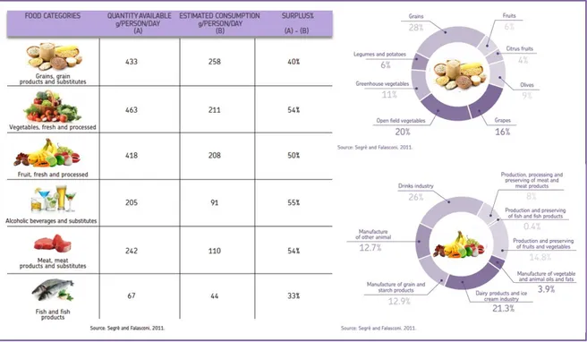
adopt stricter energy saving solutions. The production of food waste concerns all the food life cycle starting from agriculture, up to industrial manufacturing and processing, retail and household consumption. All of these stages produce large amounts of waste. The food and drink industry represents a large and economically important sector in Europe, as much as in Italy, but until the recent past, the food waste phenomenon was underestimated. Only in 2011 a study provided a quantification of the waste along the whole food supply chain: 20 million tons from the field to the point of sale (Figure 1.3; Segrè and Falasconi, 2011).
Figure 1.3. Percentages of agricultural production remaining in field and percentage breakdown of waste in
the food industry in Italy. Extracted from Barilla centre food and nutrition report on “Food waste causes impacts and proposals”, 2012.
In general the large amount of waste produced by the food industry, in addition to being a great loss of valuable materials, also raises serious management problems, both from the economic and environmental point of view. Many of these residues,
14
however, have the potential to be reused into other production systems, e.g. in the biorefineries. A sustainable agro-food industry recognizes that waste prevention, minimization and valorisation, rather than ‘end of pipe’, are the required solutions for waste management. However, strategies and technologies to secure economic and environmental solutions for an effective management of food by-product and waste still have to be implemented. In general, such streams are nowadays only partially valorised at different value-added levels (spread on land, animal feeding, composting, among others), whereas the main volumes of them are managed as waste of environmental concern with relevant negative effects on the overall sustainability of the food processing industry (Fava et al., 2013).
This happens, in general for all types of waste, also because of the lack of waste information. Usually the types and the quantity of the different components that can be found in a waste stream are often lacking or unknown, even these information are very important for the waste management planners, the local officials and material recovery facility designers. In conducting a study of local (regional, …) conditions, a variety of waste characterization methods can be used. Computer models generally use national averages for waste generation rates and other community features to calculate waste quantities. An alternative is to use materials-flow surveys based on production data for the materials and products in the waste stream, with adjustments for imports, exports and product lifetimes. Both approaches neglect some important aspects: the first does not account for local waste characteristics that can vary significantly from national or regional averages, the second never collects physical samples and it is difficult to apply when waste characteristics are evaluated at a facility such as a landfill or a treatment facility (Zeng et al.; 2005).
Collecting and characterizing samples is a good practice, which must be considered at various stages of the waste chain. First, characterization is needed to identify waste composition and properties among a waste stream. This could be useful to choose the best disposal option. Then, if the disposal option concern reuse (e.g. organic waste for
15
composting), a new characterization would be required to monitor the quality of the intervention. Furthermore, if the waste can be even valorised extracting new products (chemicals, materials, fuels, etc) from it, a deep characterization would be important to assess the quality of the originated by-product.
The already known practises to reuse waste, especially organic waste, such as composting or soil remediation, have proved to be satisfactory in many cases, if well monitored, but the new horizon of waste reuse is valorisation. Such concept comes from the past and it was mostly related to waste management, but it has been brought back to our society with renewed interest due to the fast depletion of natural and primary resources, the increased waste production and the need for more sustainable and cost-efficient waste management protocols (Arancon et al., 2013). Various valorisation techniques seem to be promising in meeting industrial demands, above all because of the need of products and processes that minimize the use and generation of hazardous substances, which is the concept of green chemistry.
There are a lot of test methods, supported by international standards, to characterize many types of waste, but a constant improvement of scientific methods is needed, moreover test methods produce waste themselves. So, further efforts are needed to make also test methods greener.
In this research thesis, Nuclear Magnetic Resonance (NMR) Relaxometry (MRR) and imaging (MRI) have been proposed, almost for the first time, to characterize organic waste materials and by-products. The strength of this technique consists in its non-destructive and non-invasive features. Magnetic resonance employs magnetic fields and radiofrequencies devices to obtain information on the nuclei on which the system is tuned. The analysed samples generally can be measured without any significant treatment and, after the measure, they can be reused. NMR is hence non-invasive and non-destructive.
The typical applications of MRR and MRI concern petrophysical and biomedical fields, so its use in environmental field is quite new. This is the reason why this work starts with
16
an optimization of the hardware and software, in this case of the NMR LAGIRN laboratory: to use NMR equipment on this kind of samples specific experimental features have been improved and adopted.
After such preliminary, but essential, work some cases study have been analysed to fully demonstrate the power of this techniques.
It has been found that MRR technique can give information on the porosity of soils treated with organic waste (in this case paper sludge). In particular the study of the microporosity (< 2 µm) has confirmed that organic matter (OM) clogs this range of pores. This evidences that high OM contents affect soils structure and they may produce negative effects on them, like anaerobic degradation, with biogas production. Then, biodegradation of compost, obtained by domestic organic waste, has been detected with both MRR and MRI, highlighting the possibility to follow OM biodegradation, establishing the maturity of compost both globally and locally, to detect eventual compost components not well degraded.
As the waste chain that leads to the production of organic waste can be further improved, other studies, which are still in progress, that conclude the experimental developments of the thesis, are focused on the reducing of organic waste, in particular of food waste.
MRR and MRI have been employed to control the efficiency of the process of fruit dehydration, which is a practice largely used to avoid food waste.
The PERFIDI filters (Sykora et al., 2007) have been employed in MRI to separate the signal in the animal meat, of the fat from that of the muscle, to improve quality controls, and to finally sell meat on the basis of its nutritional characteristics.
Then bio-oils, which are the liquid products from biomass valorisation processes, have been studied to be selected on the basis of their quality, to further propose the best way to be employed.
All these applications confirm that NMR is an innovative technique ready to be used for characterization and for quality controls on organic waste.
17
Chapter 2
18
2.1 Introduction to low-field NMR application to industrial
processes
The first Nuclear Magnetic Resonance (NMR) experiment in bulk materials date back to 1946 by Bloch, Hansen, and Packard at Stanford and by Purcell, Torrey and Pound at Harvard. The importance of their discovery was recognized, in 1952, with the Nobel Prize in Physics awarded to Bloch and Purcell. In the past 60 years NMR has bloomed in the form of different techniques: spectroscopy, relaxometry and imaging (Becker, 1993). Each technique is leader in a specific field, for example, MRI has traditionally been employed in clinical medicine, presenting a non-destructive technique for biomedical investigations, becoming today one of the most valuable clinical diagnostic tool in health care. High-resolution NMR spectroscopy provides a method of structural determination for complicated molecules such as proteins, but it also allows studies on molecular interactions including enzyme activity (Mitchell et al., 2014). MRR is strongly used in petroleum industry as a well-logging tool. In general NMR applications are still more than those currently explored.
Not all NMR techniques use the same field strength. Even if there has been a continual drive towards the use of high magnetic field, not necessarily very strong magnetic fields are desirable in all scientific contexts. At present, in several industrial fields, low-field NMR, frequently associated to permanent magnets, is to be preferred as it can provide a suitable compromise between magnetic field strength and experimental versatility for installation in industrial environments and it allows the investigation of heterogeneous materials. Moreover no cryogenic cooling is needed, economic costs are restrained, safety measures are limited (in some cases negligible) and, last but not the least, the design versatility of the magnet permits also open-access and single sided magnet arrangements. A disadvantage to take in particular care is the field stability in case of thermal fluctuations, for this reason
19
excellent thermal regulation is essential on permanent magnet low field systems designed for such experiments (Mitchell et al., 2014).
The majority of low-field experiments exploit 1H (proton) spins; the high
natural abundance and large gyromagnetic ratio of the hydrogen nucleus provides a detectable magnetization even with low-field instrumentation (Mitchell et al., 2014). For these reason it is not difficult to imagine how many applications this technique could have. There are several fields in which low-field NMR is already successful, and others in which its potentialities are not fully developed. In the world of industries it is possible to find a number of low-field NMR applications, but it is worthy to say that in the petroleum production, the food manufacture and the built environment there are the most successful ones. Low-field NMR plays two important roles in oil and gas production: well-logging tools provide access to ‘‘reservoir-scale’’ measurements of the formation fluids, whereas bench-top instruments are used to examine fluids and cored plugs of rock recovered from the reservoir. Bench-top, or laboratory, NMR systems provide fluid characterization, rock properties, and a platform for trialling new recovery methods prior to single-well pilots in the reservoir. Moreover low-field bench-top magnets are used in process control in the food industry. Total signal intensity, relaxation time distributions, or diffusion measurements (e.g. for droplet size distributions) can be evaluated and monitored. These low-field instruments can be installed to operate readily in an industrial environment. Low-field NMR and MRI has been used as a characterization and quality control tool for a wide range of food products including bread and biscuit dough, potatoes and potato starch, tomatoes, apples, processed soybean protein, and powdered food products, to cite but a few of the more recent studies. Advanced imaging techniques have been used to investigate oil and water in fried foods. Finally in civil engineering and construction industry low-field NMR is providing increased understanding of construction materials: rocks, cement and
20
wood, and the application of mobile NMR for conserving ancient buildings (Mitchell et al., 2014).
A part from these most popular applications low-field NMR can also be applied to study a whole range of physico-chemical properties and processes relevant in the field of reuse and valorisation of waste. One of the central problems is that industrial processing activities produce in Europe large amounts of by-products and waste and such waste streams are only partially valorised whereas the main volumes are managed as waste of environmental concern, with relevant negative effects on the overall sustainability. Hence the realization of regional synergies in industrial areas with intensive processing provides a significant avenue toward sustainable resource processing. To do that the need of valorise waste and by-products is becoming urgent, so wastes from one sector become the input for other sectors. The first step for applying these industrial symbiosis concepts is the identification, quantification and characterization of residues (Mirabella et al. 2013). Thanks to its non-destructive and non-invasive features, low-field NMR is a suitable candidate to explore the output of this topical sector.
2.2 Basics of NMR theory
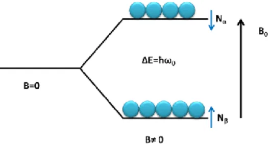
The NMR technique is based on the magnetic properties of atomic nuclei. The phenomenon of nuclear magnetic resonance occurs when the nuclei of certain atoms are immersed in a static magnetic field and exposed to a second oscillating magnetic field. Some nuclei experience this phenomenon, while others do not, depending on whether or not they possess non-zero values of a quantum mechanical property known as spin. Nuclear spin has a magnetic moment associated with it which will interact with an applied magnetic field. When a nucleus with spin, I = 1/2, such as a proton is placed in a magnetic field, two energy levels are generated. These energy levels can be
21
characterized by the magnetic spin quantum number, mI, and are separated by an
amount ΔE, which is given by:
0 0 2 h B E B (2.1)
where γ is the gyromagnetic ratio, B0 is the applied static magnetic field, h and ħ are
respectively the whole and reduced Planck constants.
The gyromagnetic ratio is a proportionality constant which relates the observation frequency for a particular nucleus to the applied field. The lower energy state, in which the nuclear magnetic moment is parallel to the applied magnetic field B0, corresponds
to mI = + 1/2. The higher energy state in which the magnetic moment is antiparallel to
B0 corresponds to mI = -1/2.
In the presence of the magnetic field the magnetic moment precesses around the applied field, with a precession frequency, Larmor frequency, which can be expressed in terms of the gyromagnetic ratio and the applied field as:
0 2 B or B0 (2.2)
where, ω is the resonant frequency in radians/second and ν is the resonant frequency in hertz. The two energy states (α,β) will be unequally populated, with the ratio of their populations given by the Boltzman equation:
E kT N e N (2.3)
22
where, Nα is the population of the lower state and Nβ is the population of the higher
state.
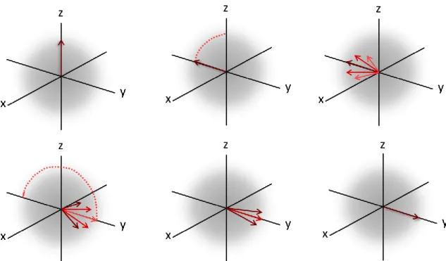
Figure 2.1 Schematic representation of the two energy states generated on protons by the B0. Although individual spins obey the law of quantum mechanics, the average behaviour of a group of ½-spins experiencing the same magnetic field strength, can be described using the classical mechanic. So it is possible to say that the population difference is dependent both on the field and the nucleus being observed, and it corresponds to a bulk magnetization (M), which is the sum of the magnetizations of the individual spins.
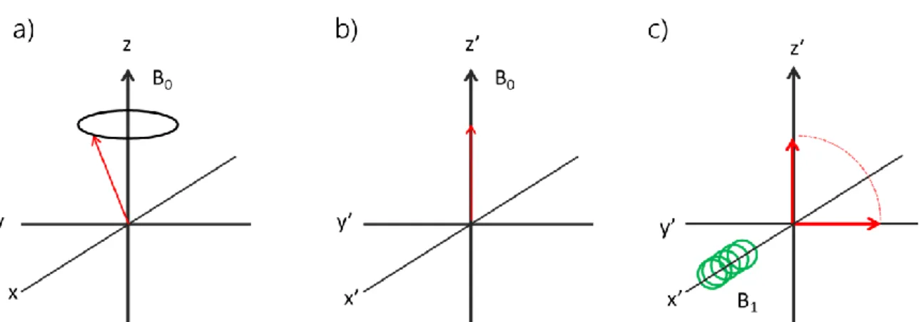
Since the magnetic moment has magnitude and direction, its behaviour in a magnetic field is usually described using vector diagrams. Initially, the bulk magnetization M, will be aligned with the applied magnetic field, till the system is perturbed (Figure 2.2 a)). The direction of the applied field is defined, for practice, as the z direction. If the induced magnetization is misaligned from the applied field B0,
a force acts on M. This magnetization is generated from nuclear spins and as a result, it behaves in a manner similar to that of a spinning top in the Earth’s gravitational field. The torque exerted by B0 on M causes M to precess around B0
(Figure 2.2 a)) at a frequency of γB0/2π hertz. This motion is known as Larmor
precession. If a coil of wire is wound around an axis perpendicular to the B0 field, the
precessing magnetization would induce an oscillating current in the coil. After necessary amplification and processing, this current becomes the NMR signal. The coordinates x, y, z are in the three-dimensional “laboratory frame of reference”.
23
From the perspective of the nuclei, these coordinates are rotating at the Larmor frequency. If the x, y coordinates are changed to those in the rotating frame x’, y’, the magnetization appears static. The net magnetization now lies along z’ and its behaviour at equilibrium is shown in Figure 2.2 b).
Figure 2.2 Behaviour of the bulk magnetization (M): a) at equilibrium in laboratory frame of reference; b) at
equilibrium in the rotating frame of reference; c) application of a B1 to displace the magnetization from the equilibrium.
In an NMR experiment, the magnetization is displaced from its equilibrium position by applying a second magnetic field B1, which oscillates at the Larmor frequency. This field
is induced from a current in a coil perpendicular to B0 and is applied for a few
microseconds. This rf field is also at the Larmor frequency. As the introduced rf radiation exactly matches the energy difference between the two states, the energy is absorbed and the nuclei are in resonance with the electromagnetic radiation. The frequency of radiation needed to induce resonance also depends on the nature of electronic shielding around the nucleus. Different functional groups or bond types in organic molecules have different electron distributions and thus their constituent nuclei resonate at different frequencies. Therefore it is possible to identify a particular functional group from its resonance frequency.
24
2.3 NMR relaxation and Bloch’s equations
The response of an isolated proton’s spin in an external magnetic field has been modelled by the classical equations of motion of a single magnetic moment. The use of classical precession picture for static fields, and of the rf induced rotation of magnetic moments in the rotating reference frame for spin ½ is justified by specific quantum analyses. In thermal equilibrium conditions the magnetization is oriented along the B0
field. In order to change the condition of the system rf pulses can be used to displace the magnetization from the equilibrium. These pulses generally rotate the magnetization of 90 ̊or 180 ̊degrees. When magnetization is rotated it is not in a stable condition, so the systems returns in the equilibrium state, this is called relaxation process.
It is possible to distinguish two processes of relaxation: the longitudinal relaxation and the transversal relaxation. The environment surrounding a nucleus is often summarily described as a lattice. The thermal motions of the lattice set up fluctuating electric and magnetic fields at the nuclei position. The interaction of the nuclear moments with these fields helps stimulate the transitions between the magnetic energy levels by emitting or absorbing energies to or from the surroundings. This process, called spin-lattice relaxation, eventually leads to thermal equilibrium. A constant interaction growth rate of the proton interactions with the lattice implies that the rate of change of the longitudinal magnetization is proportional to the difference M0 - Mz. The proportionally
constant represents the inverse of the time scale of the growth rate “T1”:
0 1 z z dM M M dt T (2.4)
25
1 1 0 0 (1 ) t t T T z z M t M e M e (2.5)Where T1 is the longitudinal, or spin-lattice relaxation time. This time reflects how
effectively the magnetic energy of the spin system is transferred to or from its surroundings. A large T1 corresponds to weak coupling and a slow approach to
equilibrium, whereas a small value of T1 indicates strong coupling and a rapid approach
to equilibrium. The transversal relaxation, which is also called spin-spin relaxation, occurs in the xy plane and it can be described by the following equation, in the rotating reference frame:
2
dM M
dt T
(2.6)
With the solution:
0 2 t T M t M e (2.7)Any process that causes the loss of transverse magnetization, including the return to the z axis, contributes to T2. The first thing that comes into consideration is the
inhomogeneity of the static field B0; recall that the magnetization vector M, when
processing in the xy plane about B0, is actually composed of all spins of the system and
all of them processing about the z axis. As a result, spins are precessing at slightly different Larmor frequencies, becoming out of phase. Moreover the decay of magnetization in the xy plane is frequently dominated by the field inhomogeneity effect, and the transverse relaxation time is generally referred to as T2* which represents
26
magnetization due to macroscopic field inhomogeneity from that due to other causes. In other words it is possible to experimentally lead to a rephasing of the spins.
In solids the nuclei are not free to move around. Hence, no matter how uniform the applied field is, the local magnetic fields due the neighbouring nuclei in the material can cause T2 to be very short.
In contrast, the nuclei in liquids move so fast that they average out the varying local fields so quickly that the only cause for transverse relaxation is the returning of the magnetization to the z axis. Thus frequently T2 equals T1 in liquids. However, T2 can
never be longer than T1.
The differential equations (2.4) (2.6) are the Bloch’s equations and they can be summarized as (in the laboratory reference frame):
0 0 1 2 1 ˆ 1 z dM M B M M z M dt T T (2.8)The general time-dependent solution for the transverse components is seen to have sinusoidal terms modified by a decay factor. The sinusoidal terms correspond to the precessional motion and the damping factor comes from the transverse relaxation effect. The longitudinal component relaxes from its initial value to the equilibrium value M0.
27
2.3.1 How to do a NMR experiment: rf pulse sequences
In a typical laboratory NMR apparatus, the sample is placed in a sample holder which is positioned between the poles of the magnet. An induction coil is looped around the sample holder such that the generated magnetic field direction is at right angles to the field magnet B0.
The coil is crossed by pulses of current at the Larmor frequency of the nucleus interrogated. The duration of these pulses determines the angle which the spins are turned apart from the direction of the B0. After the pulse is turned off, the same coil or
an additional coil is used to measure the decay or relaxation of the signal. The signal in the coil is induced by the precession of the spins around the static field in the transverse plane.
A sequence is a series of rf pulses with different duration or intensity. Rf pulses permit to rotate the magnetization of a certain angle (90 ̊ or 180 ̊). The effect of a series of rf pulses is to obtain a signal which carries information only on T1 or T2 relaxation times.
For this reason it can be said that there are T1 or T2 measurements.
If for example, a 90 ̊ pulse is used, the signal that we measure is called the Free Induction Decay (FID). The FID is largely influenced by T1, T2, magnetic field uniformity
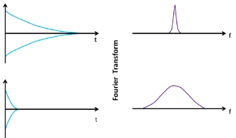
and by the presence of paramagnetic centres. Generally speaking, a long FID, when Fourier transformed to the frequency domain, gives a narrow peak at the Larmor frequency, whereas a short FID, exhibits a wide peak, indicating a heterogeneous field distribution over the sample. For example rock samples, due to very heterogeneous field, typically have a very broad peak in the frequency domain (Figure 2.4).
28
Figure 2.4 Different FIDs and the respective representation in the frequency domain.
Because of the complexity of FID interpretation, multi-pulse sequences have evolved to separate out these effects.
2.3.2 T
1measurements
To measure the longitudinal relaxation, the inversion recovery (IR) pulse sequence has the advantage to almost eliminate any T2 effects. The sequence consists of a 180 ̊
inversion pulse followed by a recovery time and then a 90 ̊ “read” pulse.
The 180 ̊ pulse inverts the magnetization vector from the positive z’ direction axis to the negative z’ directions axis. Longitudinal relaxation now occurs, causing the magnetization to go from -M0 to M0 (equilibrium). If at the time t, after the 180 ̊ pulse, a
90 ̊ pulse is applied, still along the x’ axis, M is rotated to the y’ axis. A FID results, whose initial height is proportional to Mz’ at time t. The system will return to equilibrium by
waiting at least five time the maximum T1 value. The solution for the Bloch’s equations
for inversion recovery is (Farrar & Becker, 1971):
1
/ 0
( ) (1 2 t T)
29
How much the vector grows in the +z direction during the variable recovery period also cannot be directly measured because there is no transverse component.
The purpose of the subsequent 90 ̊ pulse is to tilt the magnetization into the plane of the receiving coil where it can be acquired. A FID follows the 90 ̊ pulse, which strength is related to the growth of the magnetization along the positive z axis that has occurred since the initial 180 ̊ pulse.
A sequence of such experiments consists of a number of FIDs which are acquired at different inversion times. T1 can be computed from fitting data to equation (2.9).
Figure 2.5 Signal of a typical IR experiment.
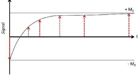
Another sequence, used to measure the T1 relaxation time, is the saturation recovery
(SR), which uses a 90 ̊ pulse followed by a 90 ̊ “read” pulse. The magnetization of the saturation recovery is described by the following equation:
1
/ 0
( ) (1 t T)
M t M e (2.10)
The popularity of the IR method is due to the fact that the dynamic range for magnetization is 2M0 as opposed to M0 for the saturation recovery. However SR has
30
the whole acquisition time (Dunn et al., 2002). This procedure is limited to cases where T2<<T1, otherwise the magnetization remaining along the y’ at time t would be rotated
to the z’ axis and would invalidate the equation to determine T1 (Farrar & Becker, 1971).
2.3.3 Field inhomogeneities and T
2measurements
The signal received by the rf detector coil is determined not just by the properties of the sample but also by magnetic interactions. The T2 relaxation is related to the
dephasing of the nuclear spins that are the result of local field inhomogeneities, among other things. The T2 relaxation mechanisms are best examined when M is first rotated of
90 ̊.
As already said, the constant B0 is not particularly uniform over the whole sample, so
the behaviour of the individual spins that contribute to the 90 ̊ rotated M (they should all be rotating together at the Larmor frequency), for one reason or another, do not rotate at exactly the same frequency. Thus in time they begin to noticeably get out of phase. In doing so, the magnitude of the vector M will decrease with time, with an exponential decay characterized by the T2* constant.
Alteration of the spin precession frequency come from the mutual interaction (spin– spin) of the proton spins (intrinsic dephasing T2). In summary the apparent decay time
will be composed, in part, of the spin–spin interactions, as well as a component due to local field inhomogeneities.
Another cause of the signal decay will be, not the dephasing, but the reorienting of the rotated spins to the direction of B0. As said before, since B0 has remained on, the
z-component of the source magnetization will increase from its initial value of zero to a final value of M, with a characteristic time constant T1 which is generally much longer
than T2 except in bulk liquids. Another source of dephasing, of interest for protons in
31
All of the sources of relaxation (or signal decay) that are not reversible are lumped into the quantity referred to as T2.
The time evolution, after a 90 ̊ pulse, is suggested in Fig. 2.6 (first row). After the M vector has been rotated by 90 ̊ it is seen at its maximum along the y’ axis. Because of the slight field differences at various parts of the sample, each of the protons may have a slightly different precessional frequency. In regions where the field is slightly larger by an amount δB the protons will precess at a slightly faster rate, γ (B0 + δB). After a time t
these protons will have advanced by an amount (γδB)t radians over the ones precessing in the nominal field B0. The converse is true for the protons that find
themselves precessing in a slightly smaller field. The spins from these various regions will tend to separate. As time progresses the spins dephase, decreasing the size of the y’ axis projection of M.
To make a measurement of T2, it is necessary to remove from the measurement any
reversible dephasing. This can be obtained by applying an Hahn echo, which is generally employed in the rf pulse sequence, the spin echo (SE). The Hahn echo is obtained when after the 90 ̊ pulse, one applies a 180 ̊ pulse.
When the 180 ̊ pulse is applied, gradually the entire arrangement of proton spins can be flipped around their position on the transverse plane so that now the slower-precessing protons will lead, and the faster ones will follow (Figure 2.6, second row). The accumulated phase of all spins experiencing a time-independent field variation will return to zero at a time called Time of Echo (TE). Therefore it is clear that all of the spins
will be realigned at the same time and the realignment is called “spin echo”.
The SE technique is limited in its range of applicability because of the effect of molecular diffusion. The refocusing of all the spins is dependent upon each nucleus remaining in a constant magnetic field during the time of echo. If diffusion causes nuclei to move from one part of an inhomogeneous field to another, echo amplitude is reduced. In general the effect of diffusion in the SE experiment is dependent upon the
32
spatial magnetic field gradients, the diffusion coefficient and the time during which diffusion can occur.
This problem can be solved by applying many 180 ̊pulses, spaced by a short half time of echo, and alternating the phase of this pulses (Farrar & Becker, 1971). This particular technique origins the pulse sequence called the CPMG pulse train after its inventors Carr and Purcell, and Meiboom and Gill. In this sequence the number of echoes which can be acquired is directly related to T2 processes.
Figure 2.6 Effects a 90 ̊pulse on M: dephasing of the spins (first row); effects of a 180 ̊pulse:
rephasing of the spins (second row).
2.3.4 NMR Relaxation in porous media
Relaxation processes of 1H fluids in porous media are important to determine a series of
petrophysical properties such as porosity, permeability, viscosity, etc. For this reason, since the 50s, applications of NMR techniques on porous media were thought for the hydrocarbons industry. Although both T1 and T2 are important measurements in porous
33
T2 has taken precedence. Unfortunately much of the early laboratory measurements,
especially in petrophysical applications, were done on T1 since it avoided the difficulties
of having a gradient-free magnetic field.
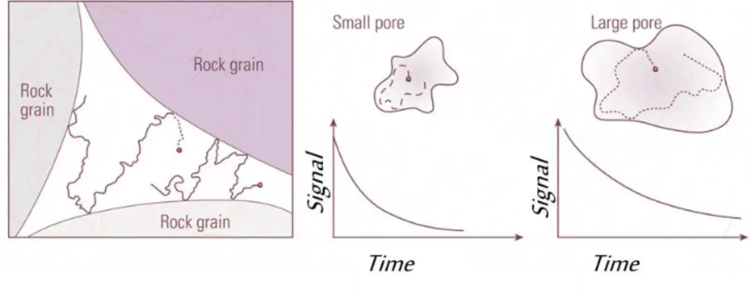
Local magnetic fields at the surfaces of the rock grains are major factor in the determination of the effective T1 and T2 for fluids in porous formations. If confined in
porous media, relaxation is often controlled by solid-fluid interactions at the surfaces of the pore space. Water molecules diffuse and eventually reach a pore wall surface where there is a finite probability that their spins are relaxed due to interactions with fixed spins, paramagnetic ions or paramagnetic crystal defects. Further transversal relaxation occurs via diffusion in local field gradients (Bayer et al., 2010). The quantity governing the interaction is the fluid diffusion length ( 6Dt ) and its relation to the pore size. T1
and T2 of confined fluids were much shorter than those of bulk fluid.
The conclusion is that the faster relaxation of the water protons must be related to the enhanced relaxation at the pore walls since the water not altered by impurities.
Brownian motion allows liquid molecules to diffuse relatively large distances during the course of NMR measurements which are on the order of a second. The distance can be estimated from the definition of diffusion, which states that the mean square distance travelled in time t, is proportional to the product of the diffusion coefficient (D) and time:
2
6
x Dt (2.11)
Since the molecular diffusion coefficient of water at room temperature is 2 × 10⁻⁵
cm2/s, a molecule can diffuse about 100 microns in a second. For many porous rocks
this is much larger than the average dimensions of a pore. This means that the molecule can have many opportunities for approaching or striking the pore wall during a measurement period. Either the spin will realign with the imposed field (a T1 process)
34
collisions before a relaxation occurs. The ability of a surface to relax the spin is called the “relaxivity” or surface relaxivity coefficient, ρ (Ellis & Singer, 2008).
Figure 2.7 Adapted from Ellis and Singer (2008). Schematization of proton relaxation inside pores
(left). Signal from a small and a large pore (right).
The total relaxation rate (1/T1,2) is, therefore, the sum of bulk relaxation (B) and surface
relaxation (S) and, for T2, of relaxation due to diffusion in field gradients (diff-FG):
1 1 1 1 1 1 total B S T T T (2.12) 2 2 2 2 1 1 1 1 total B S diff FG T T T T (2.13)
The surface relaxation term contains information of the pore system and is, therefore, further analysed. Relaxation time at the surface is determined by the residence time of the spin at the surface. The longer the residence time the higher the probability for interaction with the surface and, therefore, to relaxation. As long as this surface relaxation is slower than the transport of unrelaxed spins to the surface the fast-diffusion or surface-limited regime is fulfilled. Water molecules can pass through the pore several times before being relaxed and the magnetization decay in an individual
35
pore is, therefore, spatially uniform and depends on the surface-to-volume ratio. Surface relaxation is then related to the internal surface area S, internal pore volume V and the surface relaxivity which, as already said, is strongly influenced by paramagnetic ions, like Mn2+ or Fe3, present on the surface.
Surface limited: 1,2 1,2 1 S S T V r (2.14)
where r is the pore radius and α is the shape factor (1, 2, 3 for planar, cylindrical and spherical pore geometry). If, in contrast, the magnetic decay is controlled by the transport of the molecules to the surface the conditions of the slow-diffusion or diffusion-limited regime is met. This may be the case if pores are large or surface relaxation is strong, e.g., due to the presence of effective paramagnetic centres.
Diffusion limited: 2 1 2 1 1 S S c D T T r (2.15)
where D is the diffusion coefficient and c is a shape-dependent factor. Note that in the case of diffusion limitation T1S and T2S are equal. Relaxation times in the diffusion-limited
regime depend on temperature in the same way as the diffusion coefficient. In this case, relaxation times are not spatially uniform, which results in a multiexponential magnetic decay, even within a single pore, and relaxation is additionally dependent on pore shape (Bayer et al., 2010).
In the fast diffusion limit the decay of magnetization (either T1 or T2), from a single pore,
should exhibit a single exponential. As expected, real rocks show a slightly more complicated behaviour, which is multi-exponential. The distribution of the values of the components is related to the granular nature of the sample, hence to the pore size distribution. If the decay distribution times is viewed as a distribution of pore sizes, then
36
there is an important set of assumption: each pore is in the fast diffusion limit, the relaxing properties of the walls of all the pores are the same.
Studies (a full explanation could be find in Dunn et al., 2000) demonstrated that there is a connection between pore size, or rather the surface-to-volume ratio, and the T1 or T2
distributions. To get an actual pore size distribution, a surface relaxivity needs to be assigned and some model of the geometry needs to be assumed. If a certain geometry is assumed and the surface relaxivity is constant (usual assumption), then there will be a relation between the pore size distribution and the T1 and T2 distributions, since the
latter depend on the surface to volume ratio. Assuming a certain geometry also is equivalent to establishing a connection between a measure of the pore size and the S/V ratio. Further NMR petrophysical applications depend on a correlation between pore body size and pore throat dimension which is frequently the case for sandstones. The enhancement of the T2 decay can be due to the additional dephasing of spins due
to their diffusional displacement in a magnetic field with a gradient. The actual analytical form predicts a magnitude that depends on the diffusion coefficient. This predicted decay rate was derived for unhindered motion of the polarized molecules. For the case of, say, water molecules confined to a small pore in a porous rock, the diffusion might not be unhindered. Depending on the size of the pore and the magnitude of the self-diffusion coefficient, the molecule may be prevented from reaching its predicted mean squared displacement. In fact, for a saturated rock sample in the fast diffusion limit, it is expected that the molecules will encounter the grain surfaces a number of times during an echo spacing.
This can be exploited experimentally using a pulsed gradient spectrometer, where a gradient is actually applied to the magnetic field to enhance this effect, which can appear as a time-dependence of the self-diffusion coefficient. At very early time, D has the value expected for the unconfined fluid; its apparent value will be seen to decline as time increases and can be construed as a measure of the pore size and tortuosity. With the development of gradient tools coupled with sophisticated pulsing and
signal-37
processing tools, D and T2 can be measured simultaneously. These measurements add
a second dimension to the traditional measurements and will be very useful for determining fluid properties and perhaps wettability. The interpretation of these data may require consideration on pore system diffusion restriction (Ellis & Singer, 2008).
2.3.5 Paramagnetic impurities
Paramagnetic systems contain one or more unpaired electrons and have therefore a positive magnetic susceptibility. The more studied paramagnetic systems usually contain either free radicals or transition metal complexes in solution. The unpaired electron spins interact with nuclear spins and influence NMR spectra of liquids. Both relaxation times are greatly reduced in the presence of paramagnetic ions. The strength of the effect depends on the ion environment and specification and it is called paramagnetic relaxation enhancement. Its most palpable effect is a more or less marked broadening of the NMR resonance lines. In porous media, the paramagnetic relaxation enhancement, influences the process of relaxation inside the pore volume: when there are ions at the surface such as Mn2+ and Fe3+, the relaxivity can strongly
change. So for a quantitative estimation of pore-size distribution, the surface relaxivity of the solid must be known, which is specific for every solid fluid combination. Furthermore, surface relaxivity must be determined experimentally by comparing NMR relaxation measurements with surface-to-volume measurements using additional techniques such as optical or electron microscopy, mercury porosimetry, capillary pressure or adsorption isotherms (for example nitrogen adsorption) (Jaeger et al., 2009).
The effect of paramagnetic substances on the relaxation rate can be much stronger when they are adsorbed to the solid surface, due to the restricted molecular motion of the adsorbed species which in turn results in a longer rotational correlation time for the coordinated water molecules (Bayer et al., 2010). Nevertheless, bulk relaxation is also
38
accelerated in the presence of dissolved paramagnetic ions. This relaxation acceleration in the bulk solution is dependent on the speciation of the ion. Concluding, the acceleration of the bulk relaxation rate in comparison to pure water may give additional information on the ion environment in complex soil solutions (Bayer et al. 2010). An example of this situation is when soils saturated with water are studied: the paramagnetic ions in solution change relaxation times, and the interact with organic components (Bayer et al. 2010).
2.3.6 NMR Relaxation in biological systems
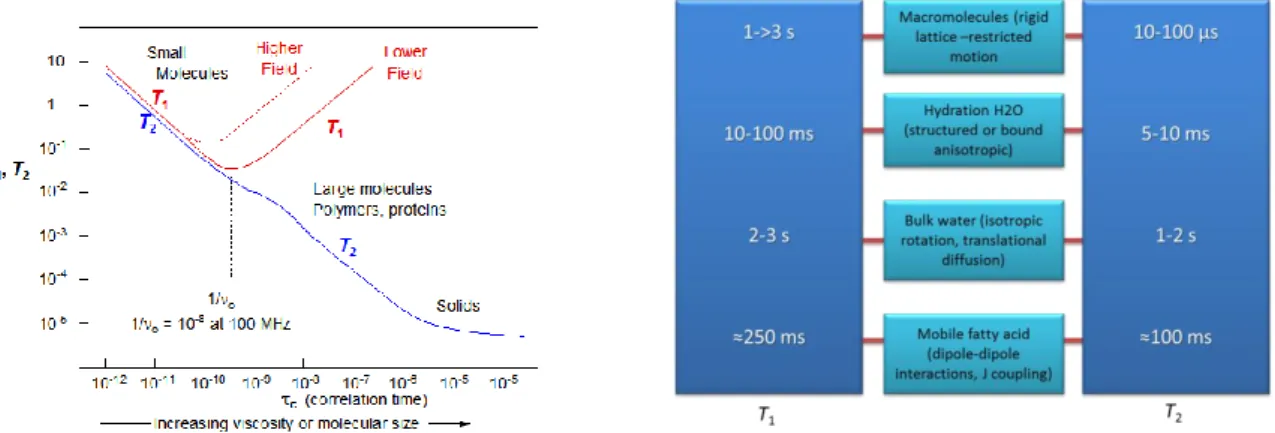
NMR applications on biological systems are at now probably more famous than those on porous media. This is largely due to the successful employment, especially of MRI, to the biomedical sciences.
Going deeper in the explanation, it is useful to speak in terms of molecular motions. For this reason the τc correlation time, should be defined as the average time between
molecular collisions for a molecule in some state of motion, and relaxation times are related to it.
As can be deduced by Figure 2.8 everything that modifies the thermal molecular motion, as for example the temperature, the viscosity, …, it will induce a variation in the relaxation times.
The BPP (Bloch Purcell Pound) theory that gives the specific plot of Figure 2.8, describes relaxation via magnetic dipole-dipole interactions (typically dominant process in liquids and tissues). It tries to explain the relaxation constant of a pure substance in correspondence with its state, taking into account the effect of tumbling motion of molecules on the local magnetic field disturbance. The theory makes the assumption that the relaxation is proportional to c
t
e
. Observing the plot of Figure 2.8 (left), it is possible to understand that from solids to liquids (increasing molecular motion) we obtain different relaxation times. If for solids T1 and T2 are very different, for a liquid
39
they become almost equal. The theory is accurate for bulk water, but not for complicated systems such as, for example, the human body. Biological systems in general are complex systems, because sum of different components, with different molecular motion. Anyway the T1 and T2 study approach give solid results, especially
when different biological species are studied separately.
Figure 2.8 Representation of relaxation times (s) vs the correlation time (s) (left); a summary of
the principal molecules with their relaxation times.
NMR techniques span the whole range of biological systems. These include: structure determination of large biological molecules, understanding biochemistry and functional behaviour of proteins and nucleic acid; cell metabolism; structure and function of tissues: imaging, metabolism and function of whole organs; pharmacology; plants and agricultural sciences and several other areas of life sciences. The application of the 1H
NMR to complex systems as biological tissues, is mainly due to the large abundance of water inside them. Broadly speaking, one can say that the cellular metabolism is strictly related to the water content. Furthermore not all the water of a biological system has only one physical or biological function. NMR can explain the different water roles; for example the measurements of relaxation times give information on the molecular motions, as relaxation phenomena are strictly related to the fluctuations of the local magnetic field caused by rotation and translation of the molecules.
40
Furthermore NMR can be applied to a wide range of liquid and solid matrices without altering the sample or producing hazardous wastes. Nowadays also food engineering, food processing and waste management are fields interested in applying innovative technologies able to detect the structure and the processes of the biological system. It is interesting, for example, to cite the example of food. Many foods are proton-rich, with protons originating, e.g., from water, fat, carbohydrates, and proteins 1H NMR
becomes the most common type of NMR to determine these abundant food components. These components are essential for human nutrition and also they influence the intrinsic properties of food during processing, storage, and transportation (Marcone et al., 2013).
2.5 NMR Imaging
2.5.1 The principles of images reconstruction
It follows a brief explanation of imaging methods, only to give idea of what is an image reconstruction in MRI.
With MRI is possible to determine the spatial distribution of a given component within the sample. Since nuclei process at different rates in locations where the magnetic field has changed, the position of the spins can be determined from frequency content of the resulting MRI signal. Furthermore the signal is the Fourier Transform (FT) of the spin density. The coverage of k-space, that will be later defined, is pivotal to reconstruct an image of a sample by the inverse FT techniques.
The signal can be represented as:
jk xx x S k x e dx
(2.16)41
If the Fourier transform in known, the ρ(x), which represents the spin density, is given by the inverse FT:
1
2 x jk x x x x S k e dk
(2.17)This is a one-dimensional example, with the choice of a x direction, but other directions could be chosen.
It is impossible to obtain S(kx) as a function of continuous kx. Instead S(kx) is measured
only at a finite number of sampling points. To demonstrate how discrete samples of the signal can be used for image reconstruction, let’s assume that S(kx) is measured at N
locations:
2 /
x x
k n L (2.18)
Where -N/2 ≤ n < N/2, and N is assumed to be even; Lx is a positive constant, known
as field-of-view (FOV), which defines the size of the imaged region.
By substitution, it is possible to define the reconstructed image intensity, I, as the inverse discrete FT of the signal:
( /2 ) 1
2 / /2 1 / n N j np N n N I p N S n e
(2.19)Where -N/2≤p<N/2. Since S(n)=S(kx(n)), substituting S(n) with the complete expression
of S(kx(n)), it is possible to obtain the relationship between the spin density and its
42
p
I p x PSF x x dx
(2.20) Where xp pLx /N and
/ sin / sin / x j x L x x e Nx L PSF x N x L (2.21)It follows that the image intensity is given by the convolution of the ρ(x) and PSF(x), known as point-spread function, where PSF(x) represents the image of a point source described by the Dirac delta function.
These results can be generalized to describe Fourier reconstruction from discrete samples in two or three dimensions.
Image intensity is the sum of weighted elements ρ(x)dx with PSF(x) as the weighting function. Furthermore, spatial resolution is the minimum distance between two points in an object at which they can still be distinguished from another in the image. δx can be defined as the effective width of a point-spread function:
/2 /2 1 0 L L x PSF x dx PSF
(2.22) Using PSF definition: / x x L N (2.23)PSF oscillates such that its maximum at the origin x=0 and rapidly decreases with increasing distance from the origin.
43
Figure 2.9 Point spread function representation.
Since PSF is a periodical function with period Lx, the reconstructed image intensity I(p) is
defined by a sum of the equally weighted object intensities at:
x x pL x mL N where m 0, 1, 2,... (2.24)
This phenomenon, aliasing, results from discrete sampling of S(k) and in general prevents complete recovery of f(x). However, under the circumstances typical for MR imaging the object has a limited spatial extent such that:
0 / 2 / 2 0 f x a x a f x otherwise (2.25)Aliasing can be fully recovered by satisfying the Nyquist criterion for the sampling interval Δk: 2 k a (2.26)
It follows that in order to prevent aliasing the selected FOV Lx should be equal to or
44
2.5.2 K-space
It is most useful to formulate imaging arguments in terms of image and data space. The inverse FT implies that the spin density can be reconstructed from the signal, if the latter is collected over a sufficiently large set of k values.
Spatial position is encoded in the reciprocal k-space signal I(k) and the image amplitude is obtained from the FT of I(k); k-space is therefore the Fourier inverse of real space. The variation of the angular frequency if the spins is defined by:
r
B0 g r
(2.27)
which is related to the applied magnetic field gradient vector g (in the laboratory reference frame), and it is written as 3D extension.
When k-space data are acquired on resonance in the rotating frame, the voxel intensity is obtained by the 3D FT of I(k) such that:
exp
2
I r
I k j k r dk (2.28)(Mitchell et al., 2014)
2.5.3 Frequency and phase encoding
In practice MRI is most frequently performed by using a sequence of pulsed magnetic field gradients which are applied during a FID or a SE to ensure that the signal is given by FT of the transverse magnetization in the sample. At this stage two basic imaging techniques for Fourier encoding must be described: frequency and phase encoding.
45
Frequency encoding is implemented by acquiring signal in the presence of an external magnetic field gradient, whose purpose is to make the Larmor frequency of nuclei spatially dependent during signal acquisition.
The signal acquired is composed of components with frequencies from a narrow range, known as the signal bandwidth, around the Larmor frequency ω0 at the centre of the
FOV.
Two-dimensional spatial encoding is achieved using an additional gradient, the phase-encoding gradient, which is perpendicular to the frequency-phase-encoding gradient.
As a result of the frequency and phase encoding the NMR signal in a two-dimensional case is given by 2D Fourier transform of the magnetization:
, jkx n x j y , jkx n x jk yy xy xy S
M x y e dxdy
M x y e dxdy (2.29) Where:kx
n G0 wn and ph t t y y t k G dt
; with τw, dwell time equal to the ratiobetween the acquisition time and the number of samples.
Phase encoding requires repetitive excitations of the transverse magnetization in the sample in order to collect signals at different values of ky. In the initially proposed
phase-encoding scheme, changes in ky were achieved by varying the duration of the
phase encoding gradient while keeping its strength constant. A more common approach is to vary the strength of the phase-encoding gradient in a step-like fashion. In this case the signal obtained with frequency and phase encoding can be written as:
, , jkx n x jky m y
xy
S n m