Analysis of some degenerate quadruple collisions

UNIVERSITAT DE BARCELONA FACUL TAT DE MATEMÁTIOUES

ANAL YSIS OF SOME OEGENERATE

QUADRUPLE COLLISIONS

by Caries Simó and Ernesto

Lacomba

Analysis of some degenerate q11adruple collisions Caries Simó* and Ernesto Lacomba**

* Facultat de Matematiques, Universitat de Barcelona, Spain. ** Departamento de Matemáticas, Universidad Autónoma Metropolitana,

México.

Abstract.- We consider the trapezoidal problem of four bodies. This is a special problem where only three degrees of freedom are invol-ved. The blow up method of McGehee can be used to deal with the qua-druple collision. Two degenerate cases are studied in this paper, the rectangular and the collinear problems. They have only two de-grees of freedom and the analysis of total collapse can be done in a way similar to the one used for the collinear and isosceles pro-blema of three bodies. We fully analyze the flow on the total colli-sion manifold, reducing the problem of finding heteroclinic connec-tions to the study of a single ordinary differential equation. For the collinear case from which arises a one parameter family of equa-tions the analysis for extreme values of the parameter is done and numerical computations fill up the gap for the intermediate values. Dynamical consequences for possible motions near total collision as well as for regularization are obtained.

§1. Introduction. The trapezoidal problem of four bodies consists in the description of the motion of four particles of mases m

1,m2 = m

1,m3,m4=m3 with initial coordinates (a,b), (-a,b), (c,d) and • (-c,d), respectively and velocities such that the symmetry of coordi na tes is keeped for all time. We can suppose that the center of masses remains at the origin, i.e., m

1b + m3d = O. New variables K=2a, y=2c, z=b-d can be introduced (see fig. 1). The motions near quadruple collision for that problem have been partially described

fig. 1 here

in

(5).

In order to give a complete picture of the flow on the to-tal collision manifold we restrict ourselves to two degenerate ca-ses: the rectangular and the collinear. In the first the four maeses

-1-are equal and a=c, b=d. In the second one has b=d=O but we ~ti 11 have one parameter: the mass ratio a= m

2/m1. Then the total

colli--sion manifold is two dimencolli--sional (see (6) and (1)) and the invariant manifolds associated to the cri ti cal points are one dimensional. The study can be done on the s&ne lines as the one found in (6) and (7) for the collinear three body prob!em, or in (1), [ 8 ) and (2) for the isosceles problem. However the analysis of the behavior of the invariant manifolds is done using a single ordinary differen-tial equation. A similar method was formulated in

(4)

and

(3).

§2. The rectangular case. First we set the masses equal to one for the bodies. We write down the Lagrangian

L

and the corresponding Hamiltonian

H _g

X 2 y

where the coordinates are described in fig. 2 fig. 2 here The resulting Hamilton equations are

x

_Px 2 2x

Px - ;¡:2 - ¡-3 y= Py Py - y2 3

-~

'

where ' = (x +y ) 2 2 ½ •

Let us introduce the change of variables (see

-1 y= Y' p y Y, p ' ' . y (6)): , d 3/2 d = dT = ' dt Then we have x2+v2 = l and

t

= ,-1(xp +yp ). Introducing V=XPX+

X y +YP y we get the blown up equations:

-2-x•

Y' P - XV X Py - YV P' X P' _y 2

X

2 - 2X +

½

VPX 2 y2 - 2Y +

½

VPY

0n t=O (total collision manifold C) the equations are still

regular and we shall use the descriptiol'I of the flow on C to get

information about passage near totRl collision. As we know the

chan-ge of variables is a diffeomorphism for t~O. The change has blown

up the point x=y=o to the manifold C. This has no physical meaning

nor the fact that the new time ton C is obtained by and infinite

slowing down of the physical time. However, the regulari ty of the

equations on C gives informations for small positive values of

t and this has a clear physical importance.

u

the equations of the e2ergy is V

and we get V' U

-2 .

The equilibrium points are u

e

and V ±18/2"+4.

e

o

where

2+4✓2

We introduce a new change of coordinates: X

and therefore

cos 8, Y =sin 8

X' = -sin

e.e•

But p2 = p2 + p2 _{2U and Arg}

X y

=

v.

Therefore

P X = P cos y After substitution we have

8' = ±/2V'

P -XV

8.

_x_

sin 8 +

allow us to write Pcos(y-8)=

p = y

V cos e - ¡---¡;2:v2 sin

e •

V'=U(e)-~2 ' U(e) = c;se + sJ!e + 2

that\,we integrate from

unstable manifold W~

8 = w/4, V IB✓'l + 4 on to obtain the

of the lower equilibrium point A (see fig. 3).

Now we have several possibilities for studying the equations of the

manifold. We can obtain d8/dV (see 13) or we can use the are par~

meter o along W~ as independent variable. The new equations are

-J-dV = (1 + 2/V')-½

da ±(1 + V'/2)-½,

avoiding all the singularities. The change of sign in d8 is

produ-da ced when 8=0 or w/2.

fig. 3 here

§3. Numerical computations and analytical estimations far the rec-tangular case. The last equations have been integrated starting .at

A up to arrivirlg to V=O (point B). The values obtained are 8(B)=

0.5877, a(B) = 4,459. It is clear, using the symmetry with

res-pect to 8 = w/4 and V=O, that to have a connection between lower,

A, and upper, D, equilibrium points requires 8 (B) be a multiple

of w/4. The value 0.5877 is quite different from O and w/4. However for people who deslikes results obtained through numerical

integra-tion we offer a proof of the fact that Ws

t

Wu that involves only

D A

inequali ties and a few evaluations of trigonometric and hyperbolic functions.

Dividing 8' by V' we have

l

ddvªI -- .2,v• = l/sec8+cosece+1-

=

J

₄

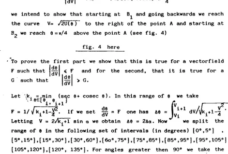
v2 we intend to show that starting at B

1 and going backwards we reach

the curve V=

/2üITT""

to the right of the point A and starting at

B₂ we reach 8 =w/4 above the point A (see fig. 4)

fig. 4 here 0

To prove the first part we show that this is true for a vectorfield

F such that

1

:~ 1 ,

F and for the second, that i t is true for a

G such that

l!!I

> G.

Let '.k1 = [min (sÍc 8+ cosec e). In this range of

e

we take

-. eE e e

i • i+l

ti

1

¡Ji

_v2

1/ Jk1+1-f. de

F = _{lf we set dV = F one has 68 =} + dV

k

+1-- •

Vi i 4

Letting V= 2 ~ sin a we obtain 68 = 26a. Now we split the

range of 8 in the following set of intervals (in degrees) [0°,5°]

{5º,15º],(15º,30º),(30º,60º],(6o0_{,75º],[75º,85°J,(85º,95°],(95º,105º)}

symmetrical with respect to 90°. The points separing intervals are e

O =0º, e1 =5º, ••• , e9=120º, \o=135°. At each one of such points

we shall compute Vi. Note that for each Vi we have two values of o, 0

21_1, 021, depending on the value of k1 used, the one re-lated to the left or right interval. Using symmetry and convexi ty k 0 sec 5° + cosec 5° = k6, k1 = 2 ✓6 = 0 k₅ = k₇, k₂ = 2+2//3 = k₄ k₈, k₃ = 2h = k 9• We set up te recurrence o₂l+l = 0 21 + (e1+1-e1)/2,

~ _{sin o 2i+l} = lki+l+l sin 0

21+2' i = O t 8, starting with o0=0. A few computations of trigonometric functions give the values a

1 ff/72, a3 = o.153246335, a5 = o.313807297, a7 = o.589183175,

ºg 0.693534686, º11 = 0.653534211, º13 = 0.501227454, º15 = .900181094 0

17 = l.335010689 and then we obtain sin 018 > 1 showing that un-der F we reach the value V=Vc to the right of polnt A.

d9

Now we proceed to study the solutlons of dV = G starting at V= O, 9= w/4. Consider the interval [a,b) e (0,w/4]. Suppose that V(a) < V(b). Then we take as 1/G J.e function /~ + sec(a)+l V~a)2 where d = b/sin b. We have l.V = 1/G (e) de. Let r¡,(m,e)=le+me2+ + _! argtanh

lf

9 if m>O an

ª

/e~me2 + b,arctg/₁

-m:

if

/iñ +me V( ) 2 -m & +m

m <o.Define g=sec(a)+l--¡-. Then AV= /ii(r¡,(~1b)-'1'(d,a)), When 9

goes from w/4 to w/2 and again to w/4 and V decreases, the variation AV !s equal to the variation obtained going from w/4 to O and again to w/4. Using the partition (w/6,w/41, (w/12, w/6],(w/36, w/12), (O,w/36) twice (the same partition used for F) we have

dV

t✓di

('I'(:! ,

9i+l) -

'/1(:!,

e_{1 )),}

where in g₁ the value V is taken w/4¡. w/6, w/12, etc. The evaluation of metrH: and hyperbolic functions gives

as } : . The values e

1 are

theJrlquired inverse

trigono-dV=3.856090805< ✓4+8✓2 IVcl proving that under G we reach 9 =w/4 on a point above A, as desi red. As a conclusion we have proved the following result.

-5-Theorem 2. l. The right part of the invariant unstable ,manifold of the lower equilibrium point

e

E (O, 11/4).

A reaches the value for

The conclusions about the remainirg part of can be obtai

ned by symmetry. After a sequence of binary collisions (of course, couples of simultaneous double collisioris) of types 1 and 2 (see

fig. 5) slightly below or above the quadruple collision point A,

the bodies escape as shown in fig. 5. A similar behavior is obtained

for left hand side collisions.

fig. 5 here

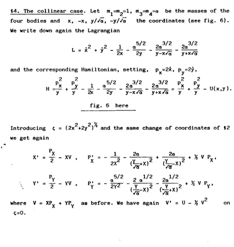
§4. The collinear case. Let m

1=m2=1, m3=m4=a be the maeses of the

four bodies and x, -x, y/ ✓a, -y/ ✓a the coordinates (see fig. 6).

We write down again the Lagrangian

L

and the corresponding

2 2 H

=-

P;c _y + py _y .2 X .2 1 ª5/2 2a3/2 2a3/2 + y - 2x - ~ - y-xra - y+xra

Hamiltonian, setting, Px=2x, Py=2y,

5/2 2a3/2 3/2 2 2

1 a 2a Px py

- 2x - _{~ - y-xro - y+x}

_ro

_{= y} + -_y - U(x,y).

fig. 6 here

Introducing t

we get again

2 2

½

(2x +2y) and the same change of coordinates of §2

PX - XV P' 1 2a 2a +

½

V PX' X'

₂

'

_2X2 < ;.¡;:+x) 2 + -X _(L..-X)2 -lrI Py 5/2 2 a 1/2 2al/2 Y'

₂

- YV P' a +

½

V py'

'

y = -

2VT -

_{( y -X)2} c...!+x,2 ro ro

where V XPX + YPY as before. We have again V' =

u -

½

v

2 on

t=O.

-6-1

Introducing X = i"Z" cose , Y

~

sin e , the equation

e•

±/2.V• is obtained.

The equilibriurn points are obtained in the following way: let

x· z

z y ;ra. From x z and letting Z= 11 x we have

a

When a ranges from O to m the parameter II does between 11

2 2 2 o

and m, where 11₀ is the zero of 11(11 -1) = 8(11 +l)

(approximate-ly 11

0=2.396812289). The minimurn value of e is given by e0=arctgra

and the critica! one by ec = arctg (11,r,;.).

In order to study the connection of the invariant manifolds

starting at points (ec, ± ✓2u(ec)) we introduce a new change of coo~

) w/2-90 w/2+90

dinates (only useful for this purpose . Let a= ₂ , b = ₂

and e= b+a sin y. Then we get

and dV dy ±nVcosy a

J ,

2 ' 2 _{( ~} 5/2 ₊ V cos y ✓2· sine 1/,/2 cos2y + _sin(a(l-sin (2a)312cos 80 v2 2 sin(e+e 0) 2 ) cos y + 3/2 2

(2a) cos ₉₀cos y

y)) + sin (a(l+sin y))

The term

2 cos J

sin(a( 1-sin y)) (and the one with the + sign in a

••similar way) has an avoidable singularity. If y= ₂

•

+ E, for instan

ce, we merely write 2 cos y sin (a( 1-siny))

4 cos2 E/2 sin(2a+)

41

where 41 = sin2 E/2 and compute sin(2a41)

41 as 2 4 3,,2 4 5414

ª3ª ,.

~ a -8 7 6

315 8 _{41 + · • ·}

arcsin (9c-b)

a is used for the

The computation must be started with

( w w ) r,:;;,,:-. dV E -

_{2 , 2 ,}

Ve ;2U(ec). In dy unstable manifold (right branch) and the

y decreasing) for the left branch.

Y = Ye

the + sign - sign (with

§ 5. Numerical computations for the collinear case. Using: the

equa-tion numerically regularized as described in 1 4 we have computed

the point Y+(Y-) where the right (left) branch of the unstable mani fold of the lower equilibrium point reaches the value V=0.

The independent parameter has been the parameter 1.1 • Table

1 shows sorne resul ts. Figure 7 offers . a rough representation of

y± as a function of a including the region of small values of

a. The computations have been done using a RK routine of fourth

order with step equal to 0.02. Sorne errors can be introduced for this value of the step for large values of a.

fig. 7 here

In order to study the possible motions on the total collision

manifold as a function of a we need the connections between the

2k-1 2k+l

equilibrium points. For y+ = - ₂- , . , k ElN or -y_= -₂- " , one

of the branches of W~ coincides with one of the branches of

w:.

For

y+ - y_ = 2k 11, k E lN, both branches meet due to the symmetry. Table

2 offers sorne values of a for which such connections are

establi--shed.

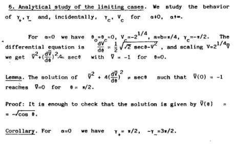
6. Analytical study of the limiting cases. We study the behavior

of y+, y_ and, inc identally, y e, V e for a+0, atm.

For a=0 we have differential equation is we get ii2+(dV)2.4' sece de 1/4

e

₀=8 =0, V =-2 • a=b=11/4, y =-11/2. The dvc l e 2 c

1/4-de = ₂

J

l'l sece-V , and scaling V=2 V

Lemma. The solution of

with ii = -1 for 8=0.

- 2

ii2 + 4(dV) ~ sece

de such that V(O)

react'tes 11=0 for e = w/2.

Proof: It is enough to check that the solution is given by V(e) = -leos

e.

Corollary. For a=0 we have y+= ,r/2, -Y_=3,r/2.

µ a _Ye V y y µ a _Ye V y y e +

-

e +

-2.39682 .000008 -1.4718 -1.1892 1.5712 -4. 7120 3.3 1.24254 .2775 -5.0787 7.4640 -6.5645 2.39685 .000036 -1.4244 -1.1894 1.5729 -4.7119 3.4 1.43195 .3126 -5.5993 8.1957 -6.8339 2.3969 .000086 -1.3886 .;l.1896 1.5752 -4.7118 3.5 1.63314 .3442 -6.1455 8.7929 -7.1057 2.397 .000183 -1.3501 -1.1900 1.5789 -4.7116 3.6 1.84650 .3729 -6.7191 9.2465 -7.3841 2.398 .001155 -1.2179 -1.1940 1.6041 -4.7107 3.7 2.07239 .3992 -7.3219 9.6424 -7.6717 2.400 .003103 -1.1153 -1.2019 1.6416 -4.7093 3.8 2.31119 .4233 -7.9556 10.016 -7.9690 2.402 .005055 -1.0534 -1.2099 1.6733 -4.7082 3.9 2.56326 .4457 -8.6220 10.385 -8.2741 2.406 .008966 - .9692 -1.2259 1.7297 -4.7064 4.0 2.82898 .4666 -9.3229 10.761 -8.5845 2.412 .014856 - .8833 -1.2498 1.8054 -4.7044 4.5 4.37492 .5531 -13.410 12.715 -10.578 2.420 .022752 - .8011 -1.2815 1.8977 -4.7026 5.0 6.31619 .6195 -18.648 15.986 -13.400 2.430 .032692 - .7237 -1.3212 2.0055 -4.7013 5.5 8.69752 .6730 -25.294 18.383 -15.688 2.438 .040698 - .6736 -1.3529 2.0882 -4.7011 6.0 11.5634 .7176 -33.628 22.057 -19.281 2.45 .052802 - .6106 -1.4002 2.2087 -4.7018 6.5 14.9582 .7556 -43.946 24.966 -22.134 1 2.46 .062974 - .5660 -1.4396 2.3070 -4.7034 7.0 18.9261 .7887 -56.564 28.993 -26.150 ~ 1 _{2.47 .073226 - .5266 -1.4789 2.4043 -4.7057 7.5 23.5114 .8178 -71.813 32.716 -30.459} 2.48 .083555 - .4913 -1.5182 2.5008 -4.7089 B.O 28.7583 .8438 -90.042 37.139 -34.200 2.49 .093965 - .4592 -1.5575 2.5969 -4.7128 8.5 34.7109 .8672 -111.616 41.624 -38.698 2.5 .104456 - .4297 -1.5967 2.6930 -4.7174 9.0 41.4134 .8883 -136.917 46.709 -43.730 2.6 .213869 - .2215 -1.9896 3.6463 -4.8028 9.5 48.9100 .9077 -166.343 50.925 -47.973 2.7 .331810 - .0904 -2.3877 4.5299 -4.9564 10.0 57.2446 .9254 -200.308 56.344 -53.323 2.8 .458723 .0051 -2.7955 5.1956 -5.1746 11.99 99.5948 .9838 -389.219 78.643 -75.591 2.9 .595040 .0800 -3.2163 5.6878 -5.4415 12.00 99.8476 .9841 -390,416. 78.726 -75.671 3.0 .741177 .1414 -3.6528 6.1072 -5.7289 12.01 100.1008 .9843 -391.616 78.808 -75.755 3.1 .897541 .1933 -4.1074 6.5080 -6.0150 20.0 467.9 1.1196 -2610.1 191.0 -187.9 3.2 1.06453 .2381 -4.5821 6.9345 -6.2932 30.0 1584.4 1.2034 -11917.9 366.9 -363.8 Table 1

k _ºk type k _ºk .. '.type 1 .09297 -y =311/2 16 10.3230 y =1311/2 2 .36153 y-=3•/2 17 12.8688 -Y+=1311/2 3 .90788 y+-Y =411 18 13.0880 y--y =1411 4 1.3452 Y+=5•/2 19 13.3035 Y+=15-./2 5 2.2181 -y+ c=5w/2 20 16.1072 -y~=15w/2 6 2.6362 y -Y =6w 21 16.3105 y -y =16• 7 2.9986 y+.:7~/2 22 16.5115 Y+=17-./2 8 4.4984 -Y+=7•/2 23 19.5572 -y+=17w/2 9 4.8210 y--Y =811 24 19.7484 y--y =18w 10 5.1229 Y+=9w/2 25 19.9379

,,+

=19•/2 + + 11 7.0515 -Y =9•/2 26 23.215 -Y =19w/2 12 7.3237 y--Y =1011 27 23.397 y--y =20w 13 7.5859 y+=llw/2 28 23.578 Y+=21w/2 14 9.8469 -Y+=ll11/2 29 27.080 -y+=21"/2 15 10.0878 y--Y =12,r 30 27.254 y--y =22• + - + -31 27.427 y =2311/2 + Table 2

flu. 8 here

Now we study what happens for a> O sufficiently small. First of all we have, approxim~telY¡

2e = ✓a. 8 = µ ✓;;_. Therefore

1 1 µ2 2:;jt 2 2c1 o ₂ e o •

= .,... + a( - l l

2 + - -1+----:-1)a+ O(a ) and V =

-12

_;,¿-re. re. µ + µ - • e

2 2 o o

µ _

1)a + O(a ). In order to check the behavlor observed in

hgve to prove two things: y+> w/2, -y_< 3w/2.

U(e) .. 2c 2 (Jlll - + 4 µ +1 o 15 we

We start at P(V=O, 8=w/2) and follow the differential equ!

dV

¡u<el

v2

tion de= - 2- - 4 backwards.

Writting down V= -2114 /cose+ w , w(w/2)

ning first order terma we get:

O and

retal-dw w cose 2 a 3/2 coa 1/2 e 1 1 _).

de = 25/4 - - + sine sin8 (sin(8+8 ) + sin(e-e ) _{o o}

The solution of the homogeneous equation is w = C(sine)-l 2 / 5/4 and

the method of variation of the constan ta gives us de = 2 a 312 coa 112

e

(----,---,- + _ _ _ _ ) • 1 1

de (sine)(l-l/25/4) sin(e+e

0) sin(e-e0)

- -1/25/4 f:/2 de

Therefore w(ec) = -(p

0

✓a) 6c, where ~/

2= ec

rz·

Tfh:,;alue

6c can be estimated in the following way Je = + ,

where z is a small but finite quantity and so 80 z

f•/2 3/2

J

2

= O(a ).

lt remains to compute the mainzcontribution

f: .

We bound cos½e by

1 1 2sin8 J«c

1 ; put -s-in_(_8_+_8_)_ + sin(8-8 ) < sin(8+8

0

)sin(8-8

0 )

the sinus by thg angles. We iet 6c ~·r:c _4_a_3/_2_8_1_1_2_s_/_4 < 4a3/2

-:_!_

f

z

J&

&2-a po-1)ec 5/4 ( P ¡;;_¡-l+l/2 o -11--2+112514 8 and approximate

Then w(ec) 4 aµ0 _As 4µ0 _<

(l-l/2514)(µ2-l) (l-l/2514)(µ2-l)

11; 2 2

o o

< 21/4 (-+--+--) the point Q (fig. 8) is abóve the equ.!_

4 µ0+1 µ -1

librium point (ec,IJc)' showing that y+ > tr/2.

Now let us look for the point R (see fig. 8). The first order

terms for Ye give us Ye .! + ✓8( µ0-1) ª1/4. 0n _{the other side}

dV 2 11

the main term in _dy is /11/4/'Z near the left hand side colli

sion. Therefore the value of t;V from the point (ec,Vc) to R is

2/11/4/'Z (11/2 + y)= /8(µ _{e o} -1)/l'Z a 1/4 , showing that -y

-have proved the following resul t ..

Proposition 6.1. For a small enough y+> 11/2, -y_< 3w/2.

F ora arge we 1 h ave 8 11 - __! 8

O 2 la, e

= V/a514 and retaining the

tion we get · Ve = -aV2a Then dV

✓1-v

2

₁₂

a ✓2 T _g 11 < 3tr/2.We

where T is the y interval and

~

is the average value of lcosyl.

We get immediately T = 2 -l/4w2a112. We state the result, showing

good agrement with table l.

Proposition 6.2. y +y + "·

+

-For a sufficiently large y ~

+ and

Corollary 6.3. There are infinite values for which the left hand

branch of Wu coincides with the left hand branch of Ws and for

1 u

which the right hand one coincides with the right hand one and for

. u s u

which w

1

=

Wu . In the last case the left hand branch of

w

1

coin-cides with the right hand one of Ws and viceversa.

u

The first one values for which those coincidences are obtained were given in table 2.

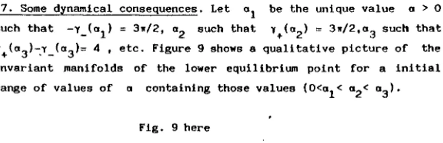
-12-§7. Sorne dynamical consequences. Let a₁ be the unique value o> O

such that -y_(o₁) = 3w/2, a

2 such that y+(o2) = 3w/2,o3 such that

y+(o₃)~y_(o₃)= 4 , etc. Figure 9 shows a qualitative picture of the

invariant manifolds of the lower equilibrium point for a initial range of values of o containing those values (O<o₁< a₂< o₃).

Fig. 9 here

The consequences with respect to orbits passing near

quadru-ple collision are now obtained easily in the same way as they where obtained for the rectangular case (see orbits type 1,2 in fig. 3).

We recall that other necessary condi tions for regularization can

U 6

be obtained (for the good values of o , Le., such that

w

1 _ Wu)in theway

introduced in (7

J.

Sufficient conditions will be given in a

forth-coming paper

(9).

From fig. 9 the way of escaping after approaching a quadruple

collision and the number of collisions taking place between central bodies or simulateous double collisions between externa! bodies can be predicted.

Pictures similar to fig. 9 can be given for the full range

of values of o. (Note that according to table 2 there is a

4 similar

for all

to º2'

k~ 6).

a

5 similar to and similar to

"k-J

8. Acknowledgements. This work was initiated when both authors were visiting the Université de Dijon (France). The first author has been partial ly supported by an Ajut a 1' Investigació of the Uni versi tat de Barcelona. The second author has been partially supported by the

Grant PCCBNAL 790178 of the CONACYT (México). The computations were

done at the Universitat Autonoma de Barcelona and at the IMPA

(Bra-sil)·;.

-lJ-Referencea

(1) Devaney, R.: In Ergodic Theory and Dynamical Syatems I, Ed.

(2) [3) [4) [5] (6) [7) [8)

A. Katok, 211, Birkhauser, Basel 1981.

Devaney, R.: These Proceedings.

Irigoyen,M.: Celestial Mechanics,

Q,

491.

Irigoyen, M. and Nahon, F.: Astron. Astrophys. 17, 286.

Lacomba, E.: To appear in Colloque Bifurcations, Théorie Er-godique et Applications, Dijon 1981.

McGehee, R.: lnventiones Math. 27, 191. Simó, C.: Celestial Mechanica, 21, 25.

Simó, C.: In Classical Mechanics and Dynamical Systema,

Mar-cel Dekker, New York, 1981.

[9] Simó, C.: Necessary and aufficient conditiona for the

geome-trical regularization of blown up singularities, to appear, 1982.

-14-m

r,

-:i -1 V X m (a,b) 9

r,,

2 V

'1

,.,,t,us ~y/~ '1aUts o(

.

1

:

1

.

.

.

.

.

.

'

-,

1 A f '') ' X ytr.: ti,

puhllc111:lor>c<( a ) J l'dldons IIMtV(U!titlU

~

de bmcelona Dlpóslt Legal 8.: 4.223-1982 BARCELONA- 1982