Koiter's asymptotic numerical methods for shell structures using a corotational formulation

(1)

6.2 Roorda frame . . . 69 6.3 Flexural-Torsional beam . . . 71 6.4 Shear plate . . . 72 6.5 L-shaped frame . . . 76 6.6 Cross–section beam . . . 77 6.7 C–section beam . . . 79 6.8 T-section beam . . . 80 6.9 Z-section cantilever . . . 81 6.10 Stiffened girder . . . 83 7 Concluding remarks 84

(3)

List of Figures

6.1 Euler beam out–plane: equilibrium path . . . 67

6.2 Roorda frame . . . 69

6.3 Roorda frame: equilibrium path . . . 70

6.4 Flexural-Torsional beam: equilibrium path . . . 71

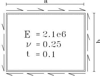
6.5 Shear plate: geometry and loads . . . 72

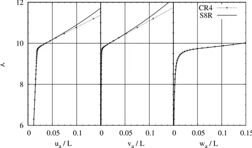
6.6 Shear plate: equilibrium paths a/b = 1.0 . . . . 73

6.7 Shear plate: equilibrium paths a/b = 1.5 . . . . 74

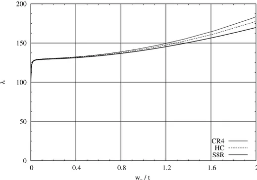
6.8 Shear plate: buckling a/b = 1.0 . . . . 75

6.9 Shear plate: buckling a/b = 1.5 . . . . 75

6.10 L-shaped frame: equilibrium path . . . 76

6.11 Cross–section beam . . . 77

6.12 Cross–section: lowests buckling modes . . . 78

6.13 C–section beam symmetric . . . 79

6.14 T–section beam L=750: equilibrium paths . . . 80

6.15 T–section beam L=450: equilibrium paths . . . 80

6.16 Z–section cantilever . . . 81 iii

(4)

LIST OF FIGURES iv

6.17 Z–section cantilever-paths . . . 82

6.18 Z–section cantilever: lowests buckling modes . . . 82

6.19 Stiffened girder . . . 83

(5)

List of Tables

6.1 Euler beam out–plane: fem convergence . . . 66

6.2 Euler beam in–plane: fem convergence . . . 68

6.3 Roorda frame: fem convergence . . . 70

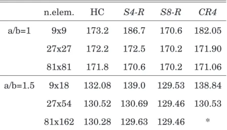
6.4 Shear plate: fem convergence . . . 73

6.5 Cross-Section: fem convergence . . . 77

(6)

List of symbols

d, dc, ϕ, ϕc Global and corotational displacements

and rotations

de, dce Vectors that collect both displacements

and rotations element-wise

g[de] Linear displacement in corotational frame

geometrically dependent on global displacement

Φe[u] Mixed Hellinger–Reissner energy functional

u Unknowns of the mixed functional dependent

of two fields: stresses and displacements

u(x, y), v(x, y) Continous displacement and

w(x, y), θ(x, y) rotational fields θ(x, y), θ(x, y)

S[u1] Second energy variation in vector format

s[u1, u2] Third energy variation in vector format

(7)

Chapter 1 Introduction

In the reviews of numerical methods used in nonlinear FE analysis [1], Riks identified two main approaches: the so–called path–following and the asymptotic analysis. Both apply to a structure subjected to an assigned loading path, usually in the form of a proportional static loading, which is described by defining its potential energy in terms of a discrete set of parameters, all collected into a configuration vector through the assumed FE interpolation.

The relationship between the configuration vector and the load mul-tiplier defining a curve (maybe composed of several separate branches) usually called equilibrium path. The aim of the analysis will be that of obtaining an accurate evaluation of its natural branch.

The basic idea in the path–following approach is to recover the equi-librium path by determining a sequence of equiequi-librium points

(8)

2

ciently near to allow the equilibrium curve to be obtained by inter-polation. The analysis develops into a step-by-step process. In each step, the new equilibrium point is determined, starting from an at-tempt value of the next equilibrium point generally obtained by an ex-trapolation from the previous step (Predictor), by an iterative Newton– Raphsson scheme which provides a convergent sequence of correction to the first attempt (Corrector), thus allowing to reduce the equilibrium error within an acceptable tolerance.

Different schemes have been proposed in literature to perform the iteration, but all of them appear as minor variations of the arc–length scheme originally proposed by Riks in [2]. A well know variant use a non linear extrapolation [3].

The main feature of the arc-length scheme is that it provides a sim-ple way to overcome limit points because the extended system remains not singular even if the Hessian becomes singular. This was a real dif-ficulty before the 1979 Riks’ paper.

To be noted that path–following analysis only needs the response vector, that is the first variation of the strain energy, to be evaluated accurately, being directly related to the equilibrium check. Conversely, the same accuracy is not actually needed for the second variation of the energy which provides the Hessian matrix because this matrix is only used as a part of the iteration process and its accuracy only influ-ences the convergence of the process. A fairly rough approximation is

(9)

3

generally sufficient for this purpose.

As a consequence, if using small steps and an appropriate configu-ration updating able to reduce, as much as possible, geometrical inco-herencies and avoid objectivity errors which could accumulate in the iterative process, the accuracy demand in the nonlinear modeling can be noticeably reduced .

The asymptotic analysis essentially corresponds to the implementa-tion of Koiter’s approach to nonlinear elastic stability [4] into a general FE context and the solution process is based on an expansion in Tay-lor’s series of the potential energy, which is characterized by fourth– order accuracy.

The actual implementation of the asymptotic approach as a com-putational tool is therefore remains of the order of that required by a standard linearized multi–modal stability analysis.

Also if the path-following strategy is a powerful approach to the postbuckling analysis of slender elastic structures [2], however it only aimes to provide the response for a single loading case, while a global evaluation of structural collapse safety, which is our principal aim, should consider all possible loadings including the deviations due to load imperfections and geometrical defects. As the single analysis is computationally quite expensive, performing a complete investigation to consider all possible imperfection shapes is difficult. Then the asymp-totic approach could be a convenient alternative for this purpose by

(10)

4

providing an effective and reliable strategy for predicting the initial post–critical behavior in both cases of limit or bifurcation points. Its main advantage lies in the possibility of performing an efficient and ro-bust imperfection sensitivity analysis even in cases of multiple, nearly coincident, buckling loads.

In fact, it provides the initial post–buckling behavior of the struc-ture, including modal interactions and jumping–after–bifurcation phe-nomena. Moreover, the presence of small loading imperfections or ge-ometrical defects can be taken into account with a negligible computa-tional extra–cost, thus allowing an inexpensive imperfection sensitiv-ity analysis (e.g see [5, 6]).

Furthermore, we can also extract information about the worst im-perfection shapes [7, 8] we can use to improve the imim-perfection sensi-tivity analysis or for driving more detailed investigations through spe-cialized path–following analysis [9].

While being less diffuse than path–following approaches within com-putational mechanics (maybe because of its high demands in terms of modeling accuracy)

The asymptotic approach is based on a fourth–order expansion of the strain energy. Thus, a careful tuning of both the continuum model and its finite element implementation is needed, to obtain accurate results, and a coherent evaluation of the kinematical relationship, at least until the fourth–order strain energy variations, is necessary [10].

(11)

5

This is an unusual requirement (path–following analysis only needs second–order accuracy for recovering the elastic response vector and the tangent stiffness matrix when a corotational or updated Lagrangian description is used), but it is important for the reliability of the re-sults , particularly in cases where the buckling is not followed by a significant stress redistribution [11]. Geometrically exact (or, at least, fourth–order accurate) strain models are generally too complex to be used in FEM analysis or are unavailable. Conversely, current model-ings, based on technical simplifications, fail to represent the strain en-ergy as uninfluenced by rigid motions, which is an essential objectivity requirement for the analysis. To overcome this difficulty, an external tool able to provide a coherent, fourth–order accurate, description of the rigid motion of the element is needed. The corotational approach (CR) [12, 13] appears to be suitable for this goal and will be exploited in this work.

A general strategy to recover objective nonlinear structural FE mod-els based on corotational description and aimed to Koiter asymptotic approach has been discussed in the paper [14]. The corotational de-scription has been used as a general tool to satisfy the objectivity re-quirement by referring each element to a local frame which moves (rotates) with the element, thus filtering its rigid motion. In this de-scription, the nonlinearity of the problem derives essentially from the change of reference, from the global fixed frame to the local one, the

(12)

6

strain energy being governed by their relative rotations. The great advantage of the method consists in the discretization phase of the process. The construction of the FE model, for the smallness of the displacements and rotations in the corotational frame, is the same of the linear elastic case, with great advantage in term of simplicity and of reuse of standard FE library. The main difficulty is in the deter-mination of the relationship between finite element parameters in the corotational frame and the corresponding quantities in the fixed global frame. In particular, in finite kinematics the presence of finite rota-tions noticeably complicates the algebra for obtaining kinematics ex-pressions.

Frame invariance in the element definition can be recovered by re-ferring the interpolation to a corotational framing moving with the el-ement in such a way to filter its rigid rotation. This approach, we call corotational interpolation, has been discussed in detail in [14].

It is worth mentioning that a mixed extrapolation is generally con-venient to avoid the so called nonlinear locking phenomena [15–17], so configuration u, used in the previous equation, usually collects both displacements and stresses.

The use of a mixed format such as that described in eqs. (1)–(4), where stresses are defined separately and determined numerically di-rectly exploiting equilibrium equations, avoids this interaction and no-ticeably improves the convergence without any need to decrease the

(13)

7

step length more than strictly required for an accurate description of the equilibrium path (see [17], for a detailed discussion).

Within an asymptotic approach, coupled with a mixed FEM rep-resentation in stress–displacement variables [16], the overall picture changes. All quantities which define the configuration state are ob-tained through a direct extrapolation, thereby reducing or completely eliminating, the need for an updating process. Nonetheless, we need an accurate evaluation for the first four variations of strain energy. The paper fouses on this goal which is reached by referring to a vec-torial parametrization of the rotation [?, ?] and deriving explicit ex-pressions for the first four derivatives of the corotational transforma-tion. When combined with a second order accurate local description of the strain energy, this allows a rather simple evaluation of the re-quired energy variations which is completely free from both extrapola-tion and interpolaextrapola-tion locking [?]. To show the effectiveness of the pro-posed approach, it was implemented in a simple case of assemblages of 3D Reissner beams. This context was chosen because it both al-lows an easy comparison with reference ”exact” results and, due to the low stress redistribution in the postbuckling range, is very sensitive to the objectivity of the strain energy description and thus convenient for checking the potential accuracy of the approach.

The work is organized as follows: after this brief introduction in the problem a presentation of the general features of Koiter’s asymptotic

(14)

8

analysis (chapter 2) also is given a short review of 3D rotation algebra. The energy variations, based on a corotational description are de-rived (chapter 3) and a complete description of the procedure needing to obtain a general and element independent framework for the Koi-ter’s analysis is given.

In order to show how a new finite element can be casted in the Koi-ter’s framework an high-performance shell finite element is described (chapter 4). This element is based on a mixed stress formulation and with a good behavior in the linear/elastic case. Here, a quadrilateral 4-node finite element (6 displacement dofs per node) is used. In partic-ular, a displacement scheme, involving the Allman drilling rotations, is used for the in-plane behavior ( [?, ?]), as well as a linked displacement interpolation is used for the out-plane behavior (see [?, ?] suitable also for thick plate analysis. The stress resultants approximation is ruled by the minimum number of parameters, both for the in-plane and the out-plane part.

The casting in to nonlinear asymptotic framework is showed (chap-ter 5) by only identifying the local variables whit the global ones and by choosing a suitable corotational frame reference fo the element.

Several numerical results are presented and discussed (chapter 6) showing the effectiveness and robustness of the proposed approach. In particular, the accuracy in reproducing the nonlinear equilibrium path in both cases of monomodal and coupled multimodal buckling is shown

(15)

9

by comparison with the commercial code ABAQUS [?] and the asymp-totic code KASP [?].

Finally, a conclusive discussion (chapter 7) about the work, the re-sults and about the possible topics for further research is reported.

(16)

Chapter 2 The Koiter’s asymptotic

numerical method

It has been described in detail in many papers (e.g. see [?,?,5,11,16–29] and references therein), thus it only needs to be briefly summarized here. Note that this approach can provide a very accurate recovery of the equilibrium path, as it derives from both numerical testings and theoretical investigations (e.g. Brezzi and al. [?], by discussing the sim-plest version of the method described in [?], derived an error estimate of O[ξ5_{] for the limit load value). Conversely, it makes great use of}

information attained from a 4th–order expansion of the strain energy and then requires a 4th–order accuracy be guaranteed in the struc-tural modeling in order to obtain an appropriate evaluation of each term of the expansion. Even small inaccuracies in this evaluation,

(17)

2.1 Outline on numerical formulation 11

riving from geometrical incoherencies in the higher–order terms of the expansion of the ε[d] law or in its finite element representation, signifi-cantly affect the accuracy or the solution and can make it unreliable. It is also very sensitive to the format used in the extrapolation, to avoid extrapolation locking (see [?] for a discussion about this topic), and the use of a mixed equation format is generally needed to obtain a robust implementation.

2.1 Outline on numerical formulation

We consider a slender hyperelastic structure subject to conservative loads λˆp increasing with the amplifier factor λ. The equilibrium is ex-pressed by the virtual work equation:

Φ0_{[u]δu − λˆ}_{pδu = 0 , ∀ δu ∈ T} _(2.1)

where u ∈ U is the field of configuration variables, Φ[u] denotes the strain energy, T is the tangent space of U at u and a prime is used for expressing the Frech`et derivative with respect to u. We assume that U will be a linear manifold so that the space of virtual displacements T will be independent of u.

Eq.(2.1) defines a curve in the (u, λ) space, the equilibrium path of the structure, that can be composed of several branches. We are usually interested in the branch starting from an initial known equilibrium

(18)

point {u0, λ0} and without any loss of generality we can consider u0 = 0,

λ0 = 0.

The asymptotic method provides an approximation of the equilib-rium path by performing the following steps:

1. The fundamental path is obtained as a linear extrapolation, from a known equilibrium configuration:

uf[λ] := λˆu (2.2)

where ˆu is the tangent evaluated at {0, 0}, obtained as a solution of the linear equation

Φ00

0uδu = ˆˆ pδu , ∀δu ∈ T (2.3)

and a pedex denotes the point along uf _{which the quantities are}

evaluated, that is Φ00

0 ≡ Φ00[uf[λ0]].

2. A cluster of buckling loads {λ1· · · λm} and associated buckling

modes ( ˙v1· · · ˙vm) are defined along uf[λ] by the critical condition

Φ00_[uf_[λ

i]] ˙viδu = 0 , ∀δu ∈ T (2.4)

Buckling loads are considered to be sufficiently close to each other to allow the following linearization

(19)

λb being an appropiate reference value of λ (e.g. the first of λi or

their mean value). Normalizing we obtain Φ000

b u ˙vˆ i˙vj = −δij, where

δij is Kroneker’s symbol.

3. The tangent space T is decomposed into the tangent V ≡ { ˙v =P_iξi˙vi}

and orthogonal W ≡ {w : Φ000

b u ˙vˆ iw = 0} subspaces so that T =

V ⊕ W. Making ξ0 = λ and ˙v0 := ˆu, the asymptotic approximation

for the required path is defined by the expansion u[λ, ξk] ≡ m X i=0 ξ ˙vi + 1 2 m X i,j=0 ξiξjwij (2.6)

where wij are quadratic corrections introduced to satisfy the

pro-jection of eq.(2.1) onto W and obtained by the linear orthogonal equations

Φ00

bwijδw = −Φ000b ˙vi˙vjδw , wij, δw ∈ W (2.7)

where, due to the orthogonality condition, w0i= 0.

4. The following energy terms are computed for i, j, k = 1 · · · m: µk[λ] = 1 2λ 2_Φ000 b uˆ2˙vk+ 1 6λ 2_{(λ − 3λ} b)Φ0000b uˆ3˙vk Aijk = Φ000b ˙vi˙vj˙vk Bijhk = Φ0000b ˙vi˙vj˙vh˙vk− Φ00b(wijwhk+ wihwjk+ wikwjh) B00ik = Φ0000b uˆ2˙vi˙vk− Φ00bw00wik B0ijk = Φ0000b u ˙vˆ i˙vj˙vk Cik = Φ00bw00wik (2.8)

(20)

where the implicit imperfection factors µk are defined by the 4th

order expansion of the unbalanced work on the fundamental path (i.e. µk[λ] := (λˆp − Φ0[λˆu]) ˙vk).

5. The equilibrium path is obtained by satisfying the projection of the equilibrium equation (2.1) onto V. According to eqs, (2.7) and (2.8), we have (λk−λ)ξk−λb(λ− λb 2) m X i=1 ξiCik+ 1 2 m X i,j=1 ξiξjAijk+ 1 2(λ−λb) 2 m X i=1 ξiB00ik +1 2(λ−λb) m X i,j=1 ξiξjB0ijk+ 1 6 m X i,j,h=1 ξiξjξhBijhk+µk[λ] = 0 , k = 1 . . . m (2.9) Equation (2.9) corresponds to a highly nonlinear system in the m + 1 unknowns λ − ξi and can be solved using a standard path–

following strategy. It provides the initial post–buckling behavior of the structure, including modal interactions and jumping–after– bifurcation phenomena.

Once the first analysis has been performed (step 1 to 4), the pres-ence of small additional, load or displacement, imperfections can be taken into account in the postprocessing phase by adding additional coefficients to eq.(2.9), with a negligible computational extra–cost (see [?]). Further information about imperfection sensitivity analysis can be found in [?, ?, ?] and in the references therein.

(21)

2.2 Hellinger Reissner formulation 15

2.2 Hellinger Reissner formulation

We know, from previous discussions, that a mixed interpolation can be really convenient in nonlinear analysis. Compatible interpolations actually mean a loss in our full freedom in tuning the interpolation, so they hardly provide the best choice. Consider however that the as-sumption of a mixed or a compatible interpolation does not necessarily imply the use of a mixed or compatible format in the problem descrip-tion as it might seems by eqs. (??) and (??). In fact, the two formats only differ in the use of stress and displacement variables or of displace-ment variables alone. We can change from a mixed to a compatible format simply by expressing stress variables in terms of the displace-ment ones or, conversely, change from a compatible format to a mixed one by explicitly introducing the stress variables and their relations to the displacement ones.

To clarify this point, we can refer to the Hessian defined by eq.(??). By assuming an interpolation based on eqs. (??) and (??), it will be directly obtained as Km[u] := X e Ae       −He De[de] DT e[de] Ge[de, te]       (2.10a)

where matrix Ge is defined by

Ge[de, te] := ∂(DT ete) ∂de =X k · ∂Dk ∂de ¸ tk (2.10b)

(22)

Dk and tk being the k–th columns of matrix De and tk the k–th

compo-nent of vector te and summation being extended to all components of

te. That is, denoting with index G the assembled global matrices, we

obtain a mixed format Km[u] :=    −HG DG[dG] DT G[dG] GG[dG, tG]    (2.10c)

which, however, can be reduced to a compatible format by static con-densation:

Kc[u] := DTG[dG]H−1G DG[dG] + GG[dG, tG]

Obviously, this rewriting does not change the element interpolation or its behavior, but only the format of its description..

Conversely, by introducing the compatibility assumption (??), the Hessian is obtained in compatible format

Kc[u] :=

X

e

Ae(K0e[de] + Ge[de])

matrix K0e being defined by

K0e[de] :=

Z

e

Bε[s]TH[s]−1Bε[s] ds (2.10d)

However, by an appropriate setting of matrices ˜De and ˜He, the latter

can be rewritten in the form

K0e[de] = ˜DTeH˜−1e D˜e

and so, by introducing the further equation ˜te = ˜H−1e D˜e[de]de

(23)

it can be split into the same mixed format as eq.(2.10a). Also in this case, the rewriting does not change the element nature, but only the format of its description.

The mixed or compatible formats, while completely equivalent in principle, behave very differently when implemented either in path fol-lowing or asymptotic solution strategies. This is an important, even if frequently misunderstood, point in practical computations which has been widely discussed in [?,?]. By referring readers to these papers and to the general discussion given in [?] for more details, we only recall here that both numerical strategies described in Section 2 need func-tion K[u] to be appropriately smooth in its controlling variables u. In path–following analysis, its smoothness will imply having K[u] ≈ ˜K := K[u0] when u moves in the neighborhood of u0of interest, so allowing a

fast convergence of the Newton iterative process. Analogously, matrix K[u] being the Hessian of the strain energy, its smoothness implies, in asymptotic analysis, that the higher–order energy term neglected in the 4th–order expansion (??) be really irrelevant, so allowing an accu-rate recovery of the equilibrium path. We know that the smoothness of a nonlinear function strictly depends on the choice of the set of its con-trol variables, that is on the format of its description, and can change noticeably when referring to another, even corresponding, set. As a consequence, the mixed and compatible format, even if referring to the same problem, can be characterized by a different smoothness and so

(24)

2.3 On the use of 3D rotations 18

they behave differently in practice, when used within a numerical so-lution process. Actually, the compatible format is particularly sensitive to what we call extrapolation locking in [?, ?] which can produce a loss of convergence, when used in path–following analysis, or unacceptable errors in the path recovery, when used in asymptotic analysis. These inconveniences are easily avoided by changing to a mixed format.

2.3 On the use of 3D rotations

The nonlinear analysis of spatial structures depends on 3D rotations algebra. A great amount of work on this topic is available in the litera-ture see [?, ?, ?, ?, ?]).

Finite 3D rotations can be directly represented in terms of an or-thogonal tensor R that is a member of the nonlinear manifold SO(3). In coordinate representation, the rotation tensor R becomes a 3×3 orthog-onal matrix that, by exploiting the orthogorthog-onality property R−1 = RT, is a function of only three parameters. However it may not be conve-nient to express the configuration changes through variables belonging to a nonlinear manifold due to the complications involved in the suc-cessive variations (see [?]). A useful way to express R in terms of the quantities lying in a vector space is that of Rodrigues [?]:

R [θ] = I + sin θ

θ W [θ] +

(1 − cos θ) θ2 W

(25)

2.3 On the use of 3D rotations 19 W [θ] ≡ spin [θ] =       0 −θ3 θ2 θ3 0 −θ1 −θ2 θ1 0       (2.12)

which uses the rotation vectors θ = [θ1, θ2, θ3]T, θ =

p θ2

1 + θ22+ θ23

be-ing the magnitude of the rotation vector. This representation uses a minimal set of parameters, is singularity free and gives a one–to–one correspondence in the range 0 ≤ θ < 2π (see [?]). Making Rθ ≡ R[θ]

and Wθ ≡ W [θ], equation (2.11) is equivalent to the exponential map

Rθ = I + Wθ+ W2_θ 2! + . . . = ∞ X n=0 Wn_θ n! = exp(Wθ) (2.13) The inverse relation is given by

θ = arcsin ω

ω ω (2.14a)

ω being the axial vector of the skew–symmetric part of Rθ, implicitly

defined by

W [ω] = 1

2(Rθ− R

T

θ) (2.14b)

and ω the Euclidian norm of ω. By a Taylor expansion we obtain θ = (1 + 1

6ω

2₊ 3

40ω

4_{+ . . .)ω} _(2.14c)

The extraction of the rotation vector by the rotation matrix Rθ, as

de-fined by eqs. (2.14), will from now on be denoted by θ ≡ log [Rθ].

The most commonly used approach in defining structural models involving 3D rotations is to express the kinematics in terms of the spin

(26)

2.3 On the use of 3D rotations 20

variations δW which, as pointed out by Nour-Omid and Rankin [?], are the quantities associated through virtual works with the common accepted definition of moments. In this case, using eq. (2.13), the vari-ation δR of R could be expressed in terms of the infinitesimal rotvari-ations defined by the spin δW :

δR = RδW (2.15)

If the current rotation R is known, eq. (2.15) allows for a simple expres-sion of the first variations of the strain energy required by the equilib-rium condition (2.1).

Remembering that R belongs to a nonlinear manifold, the succes-sive variations of the energy quickly become increasingly complicated [?]. This does not however present a real problem in the path–following analysis, which requires the accurate evaluation of the first variations of energy with respect to the configuration variables and exploits the second variations only to define an iteration matrix to be used within a Newton–like scheme. Thus a rough evaluation of these variations, obtained through simplified formulas, can be sufficient for the analy-sis. The only difficulty in this context is related to the evaluation of the current rotation R, which requires a rather expensive multiplicative updating process. Consequently, a large amount of research has been devoted to setting up an efficient updating (see [?] for further details on this topic).

(27)

intro-2.3 On the use of 3D rotations 21

duced in [?, ?, ?, ?], allows the multiplicative updating to be avoided, but introduces an additional nonlinear relation through eq. (2.11). The main advantage is, however, the possibility of describing the configu-ration in terms of variables belonging to a linear manifold thereby al-lowing the strain energy variations to be evaluated accurately through standard directional derivatives. This is particularly useful within asymptotic analysis, where an accurate evaluation of these variations, up to fourth–order, is necessary. It becomes even more necessary when using the standard asymptotic formulation presented in section ??, which requires that the configuration manifold U be linear. Accord-ingly, the rotation vector θ will be assumed as configuration variables in the sequel. It will also be shown that, rather simple general rules can be derived in order to obtain explicit expressions for the energy variations needed by the analysis.

(28)

Chapter 3 Corotational formulation

The goal of the corotational approach is to split the element motion into two parts: a rigid and a deformational one, thus providing an easy way to recover an objective structural modeling. The rigid part is defined, on average, as the motion of a corotational frame (CR ob-server) which translates and rotates with the element from the initial reference configuration to the current one. The deformational part is the local motion seen by the CR observer, within this frame. It can be made small enough with an appropriate mesh refinement, allow-ing the differences between pointwise and element average rotations to be reduced. Since the strains depend only on the deformational part, which can be assumed to be small, they can be described using simpli-fied kinematical relationships: in particular, a linearized kinematics, as the simplest choice, or a more refined quadratic kinematics, for

(29)

23

ter accuracy. The former choice allows standard linear finite elements to be reused as recognized by Rankin [?, ?]. The latter choice requires a nonlinear description of the element, while still allowing the usual simplifying ”technical” assumptions for the element modeling, due to the assumption of small deformations.

Corotational description of motion has its origins in the polar composition theorem (see [?]). According to this theorem, the total de-formation of a continuous body can be decomposed into a rigid body motion and a local deformation. In finite element implementations, this decomposition can be performed using a local CR frame that ro-tates and translates with each element (Gauss point). The advantage is that the nonlinearity of the problem is transferred to the coordinate transformation between the fixed and corotational systems, and the lo-cal displacements can be assumed small enough, in the CR frame, to allow strains to be obtained through linear or a simplified nonlinear strain–displacement relationships, without introducing significant er-rors. In fact, the strain energy thus obtained prove to be objective with respect to rigid body motions of the element and its accuracy can be increased as required with a mesh refinement. Furthermore, we can reuse linear finite element libraries [?, ?] thereby avoiding the need for objective interpolations [?, ?, ?] as occurs in other descriptions of the body motion. Conversely, the presence of rotation matrices, which lie in a nonlinear manifold and combine with a multiplicative rule,

(30)

no-24

ticeably complicates the algebra for obtaining exact expressions for the variations of the strain energy higher than the first order ones.

The corotational approach has been widely used as a basic tool for describing the configuration changes within the incremental–iterative path–following analysis [?, ?]. In this context, it requires explicit ex-pressions for the first two variations of the strain energy. Only the first variation, used for checking the equilibrium, actually needs to be eval-uated exactly. Even a rough estimate for the second one is generally sufficient, because it is only employed for defining a suitable iteration matrix to be used within a Newton–like solution process [?]. Conse-quently research in this area has been largely devoted to representing the first corotational derivative in an easy form, and to developing ro-bust and computationally fast schemes for the iterative updating of the configuration.

By this choice, displacement interpolation can be set in the form ¯

d[s] = Bd[s] g[de] (3.1)

where vector ¯de := ge[de] is the representation of de in the corotational

system and the vectorial function g_e[·] expresses the change in the ob-server rules defined by equations (20a) of [?]. We obtain a frame– invariant interpolation rule which, even being nonlinear, allows us to decouple the internal (element) derivation of functions %e[¯de] and

(31)

25

corotational transformation ruled by g_e[de]. We need some algebra to

obtain derivatives of the nonlinear function g_e[de]. These can, however,

be obtained in standard recursive form and so are easily managed in FEM analysis, as shown in [?]. Furthermore, corotational displace-ments, ruled by ¯de, are only related to the distortion of the element and

so, by mesh refinement, they can be made small enough to allow the use of the same interpolation laws derived from the linear analysis, with-out introducing noticeable interpolation locking. The smallness of ¯de

also allows an evaluation of the strain displacement relationships %[¯d] through its Taylor expansion (see [?] for details) without any notice-able loss in accuracy. A 2nd–order expansion is usually adopted while a 1st–order can be sufficient with fine meshes. It is worth mention-ing that when usmention-ing a linear approximation, the element description will coincide, in the corotational framing, with that of linear theory, so allowing a direct reuse of standard software libraries already imple-mented for linear analysis. This is a great advantage, as pointed out by Rankin in the pioneering paper of 1988 [?]. In the sequel we will refer to this approach, which was also followed in [?] and [?], as Standard Corotational.

An alternative to the corotational interpolation, which can be used for the same purpose within path–following analysis, is provided by the so called Updated Lagrangian interpolation. Essentially, it is based on the use of an element fixed framing, which is, however, taken only

(32)

3.1 Strain energy in the CR frame 26

within a single incremental step of the analysis and is updated, once the step is accomplished, to fit the new alignment of the element. This approach is obviously simpler than the corotational one, because it does not need the computation of the derivatives of g_e[de], and so it is

fre-quently used in nonlinear analysis. Conversely, if it is coupled with a standard linear interpolation it requires very small incremental steps to avoid a loss in accuracy. Moreover, a certain care is required in the updating scheme to recover geometrical coherence, as much as possi-ble, and to avoid that the error deriving from the use of a simplified strain/displacement relationship can accumulate in the incremental process. Actually, we have to be very careful, especially in the presence of coupled buckling, because losing even minor aspects of the nonlin-ear behavior can result in the mislaying of secondary bifurcations and modal jumping phenomena within the path recovery.

3.1 Strain energy in the CR frame

Let’s assume a fixed frame with versors {e1, e2, e3} and consider the

motion described by the point displacement d[X] and rotation ϕ[X] vector fields, X being the position of the point in the reference config-uration with respect to the fixed frame. The corotational versors are defined by

(33)

where α is the rigid rotation vector and c the translation vector which defines the CR motion. Using simple geometric considerations and omitting the dependence on X, for an easy notation, the deformational local part of d[X] can be described by the expressions

dc= QT(X + d − c) − X (3.3)

where dccollects the components of the deformational displacement.

Similarly, the rotation vector of the local part of point rotation R := R [ϕ] is expressed by

ϕ_c= log(Rc) with Rc= QTR[ϕ] (3.4)

The point strain will be a function of the deformational displace-ment and rotation:

ε = ε[dc, ϕc]

Assuming that dcand ϕc are small, the constitutive laws can be taken

as linear. Then, it is possible to express the finite element strain energy, in mixed form, as Φe[u] := Z Ωe ½ σ · ε[dc, ϕc] − 1 2σ · E −1_σ ¾ dΩe (3.5)

where σ is the stress associated with the elastic tensor E to the strain and Ωe is the finite element domain. Exploiting the element

interpola-tion laws, (3.5) can be rewritten, in discrete form, as: Φe[u] = βTe%[dce] −

1 2β

T

(34)

β_e being the vector of the element stress parameters and % the asso-ciated vector of the strains, as a function of the displacement element vector dce collecting deformational displacements dck and rotations ϕck

of all k–th finite element nodes (or a relevant linear combination of them). Finally K−1

c is the Clapeyron compliance matrix provided by

the complementary energy equivalence 1 2β T eHcβe= 1 2 Z Ωe σ · E−1_{σ dΩ} e , ∀ βe, σ[βe]

Exploiting the smallness of deformational displacements, we as-sume that % can have, at most, the following quadratic expression in terms of dce:

% = %_l[dce] + %q[dce, dce] (3.7)

where %_l[dce] = Ddce is a linear relationship while the j–th component

of the symmetric bilinear quadratic part of %_q is defined as: %qj[dce, dce] =

1 2d

T

ceΨjdce , Ψj = ΨTj

with j = 1 . . . nρ, nρbeing the dimension of vector %.

The discrete expression of the strain energy (3.6) becomes Φe[u] = βTeBdce+ 1 2d T ceΨ[βe]dce− 1 2β T eHcβe (3.8a)

where Ψ[β_e] = P_jβ_eΨj. Using a linear strain measure (%q ≈ 0), it

reduces to the common expression of the linear elastic case Φe[u] = βTeBdce−

1 2β

T

(35)

3.1.1 A remark on the corotational description

Letting αe be the CR rotation vector associated to the average rigid

rotation of the element and

Q_e = R[αe] (3.9)

the CR formulation is based on two fundamental steps:

a) the definition of kinematical relationships (3.3) and (3.4) that ex-press a purely geometric nonlinear relation

dce = d0e+ dg[αe, de] (3.10)

between the element displacement vector in the CR (dce) and fixed

frames (de). We assume that dg[αe, 0] = 0, so that d0e will be the

initial deformational displacement vector for de = 0. The additive

rule in (3.10) is possible thanks to the assumption that both d0e

and dg are small.

b) a local modeling of the mechanical behavior of the structures, which is an implicitly defined expression of the strain energy of the element in terms of local CR finite element parameters, which is written in the simplified form (3.8), because of the assumption of small local displacements.

Note that the geometrical nonlinearities are essentially contained in eq. (3.10), while the local modeling only implies standard finite element

(36)

3.2 Strain energy in the fixed frame 30

procedures and, if using expression (3.8b), corresponds to a linear FEM modeling. The corotational approach then leads to an efficient way of reusing standard FEM technology in a nonlinear context.

3.2 Strain energy in the fixed frame

The CR rotation vector αewill be a function of the current displacement

vector de:

αe := αe[de] (3.11)

The explicit expression of this function will depend on the particular element which is used and is based on the best compromise between algebraic simplicity and accuracy, the latter being essentially related to the smallness of the deformational part of the motion. By substituting eq. (3.11) into (3.10), we can express dce as a function of de alone:

dce = d0e+ g[de] (3.12)

The combination of eqs. (3.8) and (3.10) allows the element energy to be expressed in terms of the element vector

ue:= {βe, de}T (3.13)

which collects all parameters defining the element configuration in a single vector and can be related to the global vector u, expressing the overall configuration of the assemblage, through the known relation

(37)

where matrix Ae implicitly contains the link constraints between

ele-ments. This allows the energy to be expressed as an algebraic nonlin-ear function of u:

Φ[u] :=X

e

Φe[u]

The asymptotic approach requires the evaluation of the 2nd_{, 3}rd _and

4th_{variations of the energy by correspondence to a configuration which}

can be either the initial u0 or the bifurcation one ub. In both cases,

through an appropriate configuration updating process, we refer to a configuration characterized by de = 0, the initial stresses and (small)

deformational displacements being described by the element vectors β_0e and d0e.

To express the strain energy variations, it is convenient to refer to the fourth order Taylor expansion of g[de] starting from a configuration

characterized by de= 0: g[de] = g1[de]+ 1 2g2[de, de]+ 1 6g3[de, de, de]+ 1 24g4[de, de, de, de]+· · · (3.15) where g_n, n = 1 · · · 4 are n–multilinear symmetric forms which express the nth Frech`et variations of function g[de].

The relevant strain energy variations are reported here, for the sim-pler case of linear local modeling defined by eq. (3.8b), and then ex-tended to the quadratic local modeling defined by eq. (3.8a).

We will denote with ui (i = 1 . . . 4) a generic variation of the

(38)

the FEM discretization and with uie = Aeui the finite element

configu-ration vector collecting both displacement and stress element vectors: uie = {βie, die}T. With the same notation u0 and u0e are the global and

element reference configuration vectors.

3.2.1 Second variations using linear local modeling

Second energy variations are used in the evaluation of the fundamental mode ˆu (through eq. (2.3)) and of the bifurcation modes ˙vi (through eq.

(2.4)). In both cases, using expansion (3.15) and the energy expression (3.8a), the contribution of the element to the energy variation can be expressed as

Φ00_eu1u2 = β1eT %1[d2e] + βT2e%1[d2e] − βT1eHeβ2e+ βT0e%2[d1e, d2e] (3.16a)

where %₁ and %₂ are defined by

%₁[dje] = Beg1[dje] %2[d1e, d2e] = Beg2[d1e, d2e] j = 1, 2 (3.16b)

and then the constant matrix that depend only from the linear el-ement Be = R ΩeP T_{DU dΩ} e and He = R ΩeP T_E−1_{P dΩ} e we can rewrite

the second energy variation as element independent:

Φ00_eu1u2 = βT1eBeg1[d2e] + βT2eBeg1[d2e] − βT1eHeβ2e+ βT0eBeg2[d1e, d2e]

in order to form the hessian of the above quantity eq. (3.16) can be rearranged in a more convenient compact form using the follows energy

(39)

equivalences:

βT

0eBeg2[d1e, d2e] = dT1eGe[r0e]d2e

where r0e = βT0eBe. Then the matrix Ge[r0e] became very simple and

fast to compute.

Introducing also the matrices L1

g_s[dje] = L1dje (j = 1 . . . s) (3.17)

in wich s is the variation order.

For the corresponding vector format of the secondary energy varia-tion can be expressed in the following format

δuTS[u1] = Φ 00 u1δu (3.18) Φ00_eu1δu = δuTSe[u1e] , Se =    −Heβ1e+ BeL1d1e LT₁BT_eβ_2e+ Ge[r0e]d2e    (3.19) and the corresponding matrix

Φ00_eu1u2 = u1eT Keu2e , Ke =   −He BeL1 LT₁BT_e Ge[r0e]    (3.20) The mixed tangent matrix of the element Ke can be directly used,

through a standard assemblage process, to obtain the overall Hessian matrix K:

Φ00u1u2 = uT1Ku2 , H :=

X

e

(40)

in wich the transfering operator from local reference configuration to the global one is:

Ae=   I 0 0 Ed 0    , Ed₀ = diag(E0) (3.22)

allowing eqs. (2.3) and (2.4) to be rewritten in matrix form. In the pre-vious eq. 3.22 the Ed

0 collect in diagonal form n times E0 that rotates

both displacement and rotations for each node in the element and I have the same dimension of the β vector. Numerically this procedure can be performed in a fast way operating block-wise trough the matri-ces.

3.2.2 Third variations using linear modeling

Third energy variations are used in eq. (2.8) for evaluating the third– order coefficients Aijkand the third–order terms of the factors µk, which

are scalar quantities obtained as variations with respect to known fields ˆ

u and ˙vi. They are also used in eq. (2.7) for evaluating the right–side of

the equation which implicitly defines the quadratic modes wij. In this

case we have to evaluate secondary force vector s[u1, u2] defined by the

equivalence

δuT_s[u

1, u2] = Φ

000

u1u2δu (3.23)

δu being a generic virtual variation and δu its corresponding discrete representation. The element contribution to the scalar expressions is

(41)

easily evaluated using the general formula

Φ000_e u1u2u3 = βT1e%2[d2e, d3e] + βT2e%2[d3e, d1e] + βT3e%2[d1e, d2e]

+ βT

0e%3[d1e, d2e, d3e]

(3.24a) where %₂[·, ·] is defined by (3.16b) and %₃[· · · ] is obtained by

%₃[d1e, d2e, d3e] = Beg3[d1e, d2e, d3e] (3.24b)

βT_0e%₃[d1e, d2e, d3e] = dT3eGe2[r0e, d1e]d2e (3.24c)

Φ000_eu1u2u3 = βT1eBeg2[d2e, d3e] + βT2eBeg2[d3e, d1e] + βT3eBeg2[d1e, d2e]

+ βT_0eBeg3[d1e, d2e, d3e]

(3.24d) When the vectorial expression (3.18) is needed, making u3 = δu, eq.

(3.24a) can be rearranged in the form Φ000_eu1u2δu := δuTese=   δβe δde    T   set sed    (3.25)

where set and sed vectors may be obtained by using already defined

operators:

set = Beg2[d1e, d2e]

sed = (Ge[r1e] + Ge2[r0e, d1e])d2e+ Ge[r2e]d1e

(3.26) The overall structural vector s is then obtained by a standard as-semblage

s[u1, u2] =

X

e

(42)

3.3 Corotational scalar variations 36

3.2.3 Fourth variations using linear local modeling

Fourth energy variations are used in eq. (2.8) for evaluating the fourth– order coefficients Bijhk and the fourth–order terms in µk. The following

general formula for the element contributions can be used. Φ0000_e u1u2u3u4 = βT1e%3[d2e, d3e, d4e] + βT2e%3[d3e, d4e, d1e]

+ βT_3e%₃[d4e, d1e, d2e] + βT4e%3[d1e, d2e, d3e]

+ βT_0e%₄[d1e, d2e, d3e, d4e]

(3.27)

where function %₄[·] is obtained by

%₄[d1e, d2e, d3e, d4e] = Beg4[d1e, d2e, d3e, d4e].

3.3 Corotational scalar variations

Using (3.16b) and (3.24b) we can calculate the variations independently to the particular element but only by (3.15) in a power-full and general way. Using (3.4) and (3.3) the generic vector g[de] can be expressed as:

g[de] =       g(1)_[d e] ... g(k)_[d e]      , g (k)_[d e] =   d (k) c ϕ(k)c    , k = 1 · · · N (3.28)

(43)

3.3.1 Nodal variations

The variations can be performed node-by-node independently of the element formulation. For the first variation at the nodal parameter we have: g(k)₁ [de1] =   d (k) c1 [de1] ϕ(k)_c1 [de1]    (3.29) g(k)₂ [de1, de2] =   d (k) c2 [de1, de2] ϕ(k)_c2 [ϕ_e1, ϕ_e2]    (3.30) g(k)₃ [de1, de2, de3] =   d (k) c3 [de1, de2, de3] ϕ(k)_c3[ϕ_e1, ϕ_e2, ϕ_e3]    (3.31) g(k)₄ [de1, de2, de3, de4] =    d (k) c4 [de1, de2, de3, de4] ϕ(k)_c4 [ϕ_e1, ϕ_e2, ϕ_e3, ϕ_e4]    (3.32)

Starting from (3.3) we can get the variations respect to Q₁[de] and

to de1evaluated at the point de = 0. The variations of a rotation matrix

will be described after the following section within the variations being R[ϕ_c] and Q[de] both of the same format.

d(k)_c1 = d(k)_e1 − Q₁[de1]X(k) (3.33)

(44)

3.3 Corotational scalar variations 38 d(k)_c3 = Q₃[de1, de2, de3]X(k)− Q2[de1, de2]d(k)e3 − Q₂[de2, de3]d(k)e1 − Q2[de3, de1]d(k)e2 (3.35) d(k)_c4 = Q₄[de1, de2, de3, de4]X(k) − Q₃[de1, de2, de3]d(k)e4 − Q3[de2, de3, de4]d(k)e1 − Q₃[de3, de4, de1]d(k)e2 − Q3[de4, de1, de2]d(k)e3 (3.36)

As well as, we can get the variations of (3.4) respect to w(k)₁ [de1] as

defined in (??) ϕ(k)c [de] = (1 +1₆w2)w[de] ϕ(k)_c1 = w(k)₁ [de1] (3.37) ϕ(k)_c2 = w(k)₂ [de1, de2] (3.38) ϕ(k)_c3 = w(k)₃ [de1, de2, de3] + w(k)₂ [de1, de2] w(k)1 [de3] + w(k)₂ [de2, de3] w(k)1 [de1] + w(k)₂ [de3, de1] w(k)1 [de2] (3.39) ϕ(k)_c4 = w(k)₄ [de1, de2, de3, de4] + w(k)₂ [de1, de2] w(k)2 [de3, de4] + w(k)2 [de2, de3] w(k)2 [de4, de1] + w(k)₂ [de3, de4] w(k)2 [de1, de2] + w(k)2 [de4, de1] w(k)2 [de2, de3] + w(k)₂ [de1, de3] w(k)2 [de4, de2] + w(k)2 [de1, de4] w(k)2 [de2, de3] (3.40)

(45)

In which the scalar w2 is the second variation of 1₆wTw in the

equa-tion ?? that for symmetry may be simplified as follows (omitting k for clearness):

w2[de1, de2] = (ϕc1[de1]Tϕc1[de2] + ϕc1[de2]Tϕc1[de1])/6

= (ϕ_c1[de1]Tϕc1[de2])/3

(3.41)

Now will be performed the variation of w = (QTR − QRT)/2, with respect the variables Q and R letting

skew(T ) := (T − TT)/2 and QT₁ = −Q₁ w(k)₁ [de1] = skew(−Q1[de1] + R1[ϕ(k)e1]) = −Q₁[de1] + R1[ϕ(k)e1] (3.42) w(k)₂ [de1, de2] = skew(−Q1[de1]R1[ϕ(k)e2 ] − Q1[de2]R1[ϕ(k)e1 ]) (3.43) w(k)₃ [de1, de2, de3] = skew(R3[ϕ(k)e1 , ϕ (k) e2 , ϕ (k) e3] − Q3[de1, de2, de3] + Q₂[de1, de2]R1[ϕ(k)e3 ] − Q1[de1]R2[ϕ(k)e2 , ϕ(k)e3 ] + Q₂[de2, de3]R1[ϕe1(k)] − Q1[de2]R2[ϕ(k)e3 , ϕ (k) e1 ] + Q₂[de3, de1]R1[ϕe2(k)] − Q1[de3]R2[ϕ(k)e1 , ϕ (k) e2 ] ) (3.44)

(46)

3.3 Corotational scalar variations 40 w(k)₄ [de1, de2, de3, de4] = skew(Q2[de1, de3]R2[ϕ(k)e4 , ϕ (k) e2 ] + Q2[de2, de4]R2[ϕ(k)e1 , ϕ (k) e3 ] + Q₂[de1, de1]R2[ϕ(k)e3 , ϕ(k)e4 ] + Q2[de2, de3]R2[ϕ(k)e4 , ϕ(k)e1 ] + Q₂[de3, de4]R2[ϕ(k)e1 , ϕ (k) e2 ] + Q2[de4, de1]R2[ϕ(k)e2 , ϕ (k) e3 ] − Q₃[de1, de2, de3]R1[ϕ(k)e4 ] − Q3[de2, de3, de4]R1[ϕ(k)e1] − Q₃[de3, de4, de1]R1[ϕ(k)e2 ] − Q3[de4, de1, de2]R1[ϕ(k)e3] − Q₁[de1]R3[ϕ(k)e4, ϕ (k) e2 , ϕ (k) e3 ] − Q1[de2]R3[ϕ(k)e1 , ϕ (k) e3 , ϕ (k) e4] − Q₁[de3]R3[ϕ(k)e2, ϕ(k)e4 , ϕ(k)e1 ] − Q1[de4]R3[ϕ(k)e3 , ϕ(k)e1 , ϕ(k)e2] ) (3.45) Variations of the nodal rotation R[ϕ(k)e ] matrices and of corotational

frame Q must be performed in order to get all complete variations scheme: Q₂[de1, de2] = ( Q1[de1]Q1[de2] + Q₁[de2]Q1[de1] )/2 (3.46a) Q₃[de1, de2, de3] = ( Q1[de1]Q2[de2, de3] + Q₁[de2]Q2[de3, de1] + Q₁[de3]Q2[de1, de2] )/3 (3.46b) Q₄[de1, de2, de3, de4] = ( Q1[de1]Q3[de2, de3, de4] + Q₁[de2]Q3[de3, de4, de1] + Q₁[de3]Q3[de4, de1, de2] + Q₁[de4]Q3[de1, de2, de3] )/4 (3.46c)

(47)

and for completeness we will report also variations of nodal rotation matrices, however it have the same format of 3.46:

R1[ϕ(k)e1 ] = spin(ϕ (k) c1 ) (3.47a) R2[ϕ(k)e1 , ϕ (k) e2 ] = ( R1[ϕ(k)e1 ]R1[ϕ(k)e2] + R1[ϕ(k)e2]R1[ϕ(k)e1 ] )/2 (3.47b) R3[ϕ(k)e1 , ϕ(k)e2 , ϕ(k)e3] = ( R1[ϕ(k)e1]R2[ϕ(k)e2 , ϕ(k)e3 ] + R1[ϕ(k)e2 ]R2[ϕ(k)e3, ϕ (k) e1] + R1[ϕ(k)e3 ]R2[ϕ(k)e1, ϕ(k)e2] )/3 (3.47c) R4[ϕ(k)e1 , ϕ (k) e2 , ϕ (k) e3, ϕ (k) e4] = ( R1[ϕ(k)e1]R3[ϕ(k)e2 , ϕ (k) e3, ϕ (k) e4] + R1[ϕ(k)e2 ]R3[ϕ(k)e3, ϕ (k) e4, ϕ (k) e1 ] + R1[ϕ(k)e3 ]R3[ϕ(k)e4, ϕ(k)e1, ϕ(k)e2 ] + R1[ϕ(k)e4 ]R3[ϕ(k)e1, ϕ (k) e2, ϕ (k) e3 ] )/4 (3.47d)

To be noted that it is omitted only the first variation of Q that de-pend on the particular chose of the corotational element frame and also its first variation. The first variation of the corotational reference will be given with the particular element used.

All the others variations can be obtained then in a powerful way by using the chain–rule derivation. Obviously, an optimized implemen-tation of these routines need to be performed in order to make perfor-mavit the algorithm.

(48)

3.4 Concluding remarks 42

3.4 Concluding remarks

As we can see in all of 3.46, 3.47, ??, ?? the dependence on element formulation it is only on the definition of Q[de] and its first variation.

Then, this scheme may be used for to derive the corotational variations for any finite element within a framework whit 6 DOF for node in-dependently of the number of nodes and of the particular linear finite element.

To be noted that the methods it is very powerful because only we need to define first variation of Q for each new element that need to be implemented. In fact, all successive variations are recursively depen-dent from these of previous order. This strong characteristic provide a fully way to generalize the corotational Koiter’s method to all kind of linear finite element already know.

(49)

Chapter 4 Linear Flat shell model

4.1 Introduction

Consider a plate referred to a Cartesian coordinate frame (O, x, y, z), with the origin O on the mid-surface Ω and the z-axis in the thickness direction, −h/2 ≤ z ≤ h/2, where h is the plate thickness. Let ∂Ω be the boundary of Ω. The first-order shear deformable theory, often called Reissner-Mindlin theory, and Plane Stress theory are employed. Thus it is assumed that

u(x, y, z) = u(x, y) + zθy(x, y)

v(x, y, z) = v(x, y) − zθx(x, y)

w(x, y, z) = w(x, y)

(4.1)

where u, v, w are the displacements along the x, y and z axes, respec-tively, and θx, θy are the rotations of the transverse normal about the x

(50)

4.1 Introduction 44

and y axes. The sign convention is depicted in Figure ??.

By refer to the plane z = 0 the compatibility equations can be writ-ten as follows

² = Dmu, χ = Dbθ, γ = Dsw + θ, (4.2)

where vectors u, θ, χ and γ collect, respectively, the rotations, the cur-vatures and the shear strains,

u =   u v    , ² =       ²x ²y ²xy      , θ =    θx θy    , χ =       χx χy χxy      , γ =    γx γy    , (4.3) and operators Dm, Db(see [?] about changing on sign) and Dsare given

by Dm =       ∂/∂x 0 0 ∂/∂y ∂/∂y ∂/∂x      , Db =       0 ∂/∂y ∂/∂x 0 ∂/∂x ∂/∂y      , Ds =    ∂/∂x ∂/∂y    . (4.4) The equilibrium equations can be obtained via the principle of virtual work in the form

D∗

mN = n, D∗bM + S = m, D∗sS = q, (4.5)

(51)

4.1 Introduction 45

moment and shear resultants,

N =       Nx Ny Nxy      , M =       Mx My Mxy      , S =    Sx Sy    , (4.6)

q and m, n are the prescribed loads in Ω and D∗ _{adjoint to D:}

D∗ = DT. (4.7)

For a linearly elastic material, the constitutive equations can be writ-ten as

N = Cm², M = Cbχ, S = Csγ, (4.8)

where Cm, Cb and Cs are the matrices of membrane, bending and

transverse shear moduli. In the isotropic case, the elasticity matrices specialize as: Cm = Eh (1 − ν2₎       1 ν 0 ν 1 0 0 0 (1−ν)₂      , Cb = h 2 12Cm, Cs = kGhI2 (4.9)

being E the Young’s modulus, G the shear modulus, ν the Poisson’s ratio and k a correction factor to account for non-uniform distribution of shear stresses through the thickness. The equilibrium problem of linear elastic shear deformable shell is ruled by Equations (4.2), (4.5) and (4.8) in Ω, together with appropriate boundary conditions on ∂Ω.

(52)

4.2 Isoparametric formulation 46

The variational formulation is based on a Hellinger-Reissner func-tional: Φ[u] = Z Ω µ σT_{ε[u] −} 1 2σ T_E−1_σ ¶ dΩ − Φext (4.10) where σ =       N M S      , E =       Em 0 0 0 Eb 0 0 0 Es      , ε =       ² χ γ       (4.11) .

The variational formulation of the problem described in terms of stress resultants and generalized displacements is

Φ[u] = −1 2 Z Ω ¡ NT_E−1 m N + MTE−1b M + STE−1s S ¢ dΩ+ Z Ω £ NT_D mu + MTDbθ + ST(Dsw + θ ¤ dΩ − Φext, (4.12)

where Πext is the work done by external (body and boundary) loads.

4.2 Isoparametric formulation

The element geometry is represented based on a 4-node scheme. A general quadrilateral element is considered in a local Cartesian system of coordinates (see Figure ??). The transformation between the local coordinates x and y and the natural coordinates ξ and η is given by

   x y    =    a1ξ + a2η + a3ξη b1ξ + b2η + b3ξη    , (4.13)

(53)

4.2 Isoparametric formulation 47 where       a1 b1 a2 b2 a3 b3      = 1 4       −1 1 1 −1 1 −1 1 −1 −1 −1 1 1                x1 y1 x2 y2 x3 y3 x4 y4          , (4.14)

being xi and yi the local coordinates of the i-th corner node. The

Jacobian J of the coordinate transformation defined by Equation (4.13) can be written as J = J0+ J1, (4.15) J0 =    a1 b1 a3 b3    , J1 =    a2η b2η a2ξ b2ξ    ,

and its determinant j is

j = det J = j0+ j1ξ + j2η, (4.16)

j0 = a1b3− a3b1, j1 = a1b2− a2b1, j2 = a2b3− a3b2.

For later convenience, the following quantities are introduced: ¯ ξ = ξ + j2 j0 ξη, η = η +¯ j1 j0 ξη. (4.17)

It can be easily verified that quantities ¯ξ, ¯η are linearly related to the local coordinates x, y through the Jacobian of the mapping (4.13)

(54)

eval-4.3 Assumed displacement 48

uated at the origin (ξ = η = 0):    x y    = JT0    ¯ ξ ¯ η    . (4.18)

Thus, for a general quadrilateral element, ¯ξ and ¯η define a skew coordinate system, as shown in Figure ??.

4.3 Assumed displacement

In order to avoid locking a linked interpolation was used in both case of in–plane ad out–of–plane displacements interpolation. All four edges of the quadrilater may be treated as 2-D beam element with shear de-formation: nij =   cos αij sin αij    = 1 lij   ∆y ∆x    (4.19) tij =   − sin αij cos αij    = 1 lij   −∆x ∆y    (4.20) lij = q ∆2 x+ ∆2y (4.21) .

The general interpolation function for any typical edge can be ex-pressed [30, 31] by:

(55)

4.3 Assumed displacement 49 u(ξ, η) = 4 X i=1 Uiui+ 4 X i=1 ∆yi 8 L ∗ i(θzj− θzi) v(ξ, η) = 4 X i=1 Uivi− 4 X i=1 ∆xi 8 L ∗ i(θzj− θzi) w(ξ, η) = 4 X i=1 Uiwi− 4 X i=1 ∆yi 8 L ∗ i(θxj− θxi) + 4 X i=1 ∆xi 8 L ∗ i(θyj − θyi) θx(ξ, η) = 4 X i=1 Uiθxi θy(ξ, η) = 4 X i=1 Uiθyi θz(ξ, η) = 4 X i=1 Uiθzi (4.22) where Ui = 1 4(1 + ξiξ)(1 + ηiη); i = 1, .., 4 (4.23) Li =      1 2(1 − ξ2)(1 + ηiη); i = 1, 3 1 2(1 − η2)(1 + ξiξ); i = 2, 4 (4.24) and j =      i + 1 i = 1, 2, 3 1 i = 4