Basins of attraction and dynamical integrity of nonlinear dynamical systems in high dimensions

(1)

UNIVERSITÀPOLITECNICA DELLEMARCHE, ANCONA, ITALIA POLYTECHNICUNIVERSITY OFMARCHE, ANCONA, ITALY

DOCTORAL

THESIS

Basins of attraction and dynamical

integrity of nonlinear dynamical systems

in high dimensions

Author:

Nemanja ANDONOVSKI

Supervisor:

Prof. Stefano LENCI Polytechnic University of Marche, Ancona, Italy

Co-supervisor:

Prof. Ivana Kovaˇci´c

CEVAS, Faculty of Technical Sciences, University of Novi Sad, Novi Sad, Serbia

A thesis submitted in fulfillment of the requirements for the degree of Doctor of Philosophy

(2)

(3)

iii

Declaration of Authorship

I, Nemanja ANDONOVSKI, declare that this thesis titled, “Basins of attraction and dynamical integrity of nonlinear dynamical systems in high dimensions” and the work presented in it are my own. I confirm that:

• This work was done wholly in candidature for a research degree at Polytechnic University of Marche, Ancona, Italy.

• Where any part of this thesis has previously been submitted for a degree or any other qualification at this University or any other institution, this has been clearly stated.

• Where I have consulted the published work of others, this is always clearly attributed.

• Where I have quoted from the work of others, the source is always given. With the exception of such quotations, this thesis is entirely my own work.

• I have acknowledged all main sources of help.

• Where the thesis is based on work done jointly with others, I have made clear exactly what was done by others and what I have contributed myself.

(4)

(5)

v

“Some dreams you know will never come true. But you keep dreaming anyway.”

(6)

(7)

vii

POLYTECHNIC UNIVERSITY OF MARCHE

Abstract

PhD School in Engineering Sciences

PhD in Civil, Environmental and Building Engineering and Architecture Doctor of Philosophy

Basins of attraction and dynamical integrity of nonlinear dynamical systems in high dimensions

by Nemanja ANDONOVSKI

One of the consequences of rich dynamics in nonlinear systems is the multi-stability, i.e. the coexistence of various stable states (attractors), which can have different ro-bustness. Typical example of stable attractors, but very unsafe for practical applica-tions, are those with riddled basins of attraction. To examine and eventually quantify this sensitivity to initial conditions, we can study the shape, size and compactness of basins. However, when the dimension of the dynamical system increases, it is no longer sufficient to analyse arbitrary cross-sections to get the global overview of the dynamics, and a full-dimensional basins have to be determined. Due to lack of analyt-ical methods, numeranalyt-ical computations are required to discover basins. Those numer-ical techniques applied to strongly nonlinear systems, with six or more state-space variables - that are main goal of this PhD thesis - demand considerable amounts of computing power, available only on High-Performance Computing platforms. With the aim to minimize computing requirements, we developed a software to adapt basin computations to small, affordable cluster computers, and with minor modifications utilizable also on larger ones. Our approach is based on Simple Cell Mapping method, modified to reduce the memory requirements, adjust integration time and overcome some discretization drawbacks. The resource intensive parts of computations are parallelized with hybrid OpenMP/MPI code, while less demand-ing operations are kept serial, due to their inherit sequential nature. The modifica-tions we advised, that address disadvantages of originally proposed method, and the parallelization, are classified under common name - Not So Simple Cell Map-ping (NSSCM). As intended, the program computes full six-dimensional basins of attraction within reasonable time-frame, with the adequate accuracy to distinguish compact parts of basins, but not to fully disclose fractal basin boundaries. Visual in-spection of results can demonstrate how some basins that look robust in some cross-sections may be very narrow or do not exist in other dimensions, directly altering the robustness of corresponding attractors. Anyhow, the proper robustness analy-sis must be performed to include entire state-space window. Robustness is quanti-fied by dynamical integrity measures, that exploit previously determined basins by, roughly speaking, computing the largest geometrical objects that can fit inside.

The whole development and computation approach, together with the results in form of basins of attraction and dynamical integrity, are the topic of this thesis, structured in a way to provide full insight into our research development. The first Chapter introduces the High-Performance Computing (hardware and software plat-forms, algorithm design methodology and overall efficiency), that is followed by the second one which deals with the serial and parallel methods to compute basins of

(8)

attraction, coronated with the main effort of our research - Not So Simple Cell Map-ping. The third Chapter introduces the concepts and defines the dynamical integrity measures, which closes theoretical part of thesis. Then, on the test system consist-ing of three coupled Duffconsist-ing oscillators, the computational efficiency and accuracy of NSSCM approach is discussed and validated by comparison with more accurate, but significantly slower Grid of Starts method.

Final chapters demonstrate applications of NSSCM and integrity analysis on two examples: sympodial tree model with first-level branches; and rotating hub with two pendulums. Dynamics of those strongly nonlinear systems is studied system-atically to demonstrate why classical stability analysis is not sufficient to uncover the properties of global behaviour. Integrity analysis and inspection of certain low-dimensional cross-sections of full-low-dimensional basins showed the complex behavior of those systems, which cannot be determined otherwise.

With the approach described in this thesis, and when sufficient computing re-sources are available, one can compute dynamical integrity for an interval of rele-vant system parameter(s) and get the most valuable representation of system safe-ness - integrity erosion profiles.

(9)

ix

Acknowledgements

First of all, I thank my parents Svetlana and Dragan, for their patience and support. Thanks to Prof. Ivana Kovaˇci´c who encouraged me not to be afraid of things never tried before, and taught me the value of dedication.

Thanks to Prof. Stefano Lenci, with whom I learned that there are no such things that cannot be done, only those we choose not to.

And, many thanks go to my friends at archery club and University who made Ancona feel like home.

For the invaluable help with High-Performance Computing, I thank Professors Franco Moglie, Polytechnic University of Marche, Ancona, Italy, and Radu Serban and Dan Negrut from University of Wisconsin, Madison, USA.

Results presented in this thesis are computed under the CINECA ISCRA C-type project IsC66 DIAHIDD, thus we acknowledge the CINECA award under the ISCRA initiative, for the availability of high performance computing resources and support.

(10)

(11)

xi

List of Figures

2.1 Flynn’s Taxonomy. . . 6

3.1 Poincaré sections for return and stroboscopic map . . . 19

3.2 Trajectory and Poincaré section of a periodic attractor . . . 20

3.3 Trajectory and Poincaré section of a quasi-periodic attractor . . . 21

3.4 Trajectory and Poincaré section of a chaotic attractor . . . 21

3.5 Fractal curve - Koch snowflake. . . 22

3.6 Basins with smooth and fractal boundaries. Riddled basins . . . 23

3.7 Cell discretization scheme . . . 26

3.8 Discretization of continuous trajectories with SCM . . . 26

3.9 Generic example of 2D mapping function. . . 27

3.10 Approximation of real trajectory with a discrete map . . . 27

3.11 Example of disconnected periodic orbits . . . 34

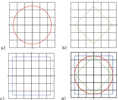
4.1 Examples of distance transform matrices . . . 39

4.2 Definition of circles for various metric spaces . . . 40

4.3 Example and comparison of integrity measures. . . 40

5.1 Test system attractors . . . 42

5.2 Impact of integration time on the SCM/NSSCM accuracy . . . 44

5.3 Comparison of the SCM/NSSCM and GoS accuracy . . . 45

5.4 Example of test system compact basins. . . 46

5.5 Cross-sections with both tangled and compact basins (example no. 1) . 46 5.6 Cross-sections with both tangled and compact basins (example no. 2) . 47 5.7 Example no. 1 of basin cross-sections with fractals and intermittency . 47 5.8 Example no. 2 of basin cross-sections with fractals and intermittency . 48 5.9 Example no. 3 of basin cross-sections with fractals and intermittency . 48 5.10 Basins with abrupt structure change (step no. 1) . . . 48

5.11 Basins with abrupt structure change (step no. 2) . . . 49

5.12 Basins with abrupt structure change (step no. 3) . . . 49

5.13 Basin compactness in various directions . . . 51

6.1 Model of sympodial tree with first-level branches . . . 54

6.2 Bifurcation diagrams for ω= (0, 3.6)and ζ =0.02 . . . 55

6.5 Bifurcation diagrams for ω= (1.35, 1.75)and ζ =0.02. . . 57

6.8 Bifurcation diagrams for ω= (2.9, 3.2)and ζ =0.02 . . . 59

6.9 STREE attractors for ζ=0.02, ω =1.45 . . . 60

6.10 STREE attractors for ζ =0.02, ω =1.53 . . . 60

(16)

6.14 Basin structure of trunk segment for ζ =0.02 and ω=1.45 . . . 64

6.15 Basin structure of left branch segment for ζ =0.02 and ω=1.45 . . . . 65

6.16 Basin structure of right branch segment for ζ=0.02 and ω =1.45 . . . 66

6.17 Basin structure of trunk segment for ζ =0.025 and ω =1.5755 . . . 67

6.18 Basin structure of left branch segment for ζ =0.025 and ω=1.5755 . . 68

6.19 Basin structure of right branch segment for ζ=0.025 and ω =1.5755 . 69 6.20 Basin structure of trunk segment for ζ =0.03 and ω=1.58 . . . 70

6.21 Basin structure of left branch segment for ζ =0.03 and ω=1.58 . . . . 71

6.22 Basin structure of right branch segment for ζ=0.03 and ω =1.58 . . . 72

6.23 Model of rotating hub with two pendula. . . 73

6.24 Bifurcation diagrams of RHUB system for ω= (0, 2.4). . . 75

6.25 Bifurcation diagrams of RHUB system for ω= (1.2, 1.65) . . . 75

6.26 Attractors for RHUB system at ω=1.4 . . . 75

6.29 Comparison of RHUB system basins computed with NSSCM and GoS 77 6.30 y0-y1basin cross-section of hub segment . . . 78

6.31 Basin structure of right pendula segment for ω =1.4 . . . 79

6.32 Basin structure of left pendula segment for ω=1.4 . . . 80

6.34 Basin structure of left pendula segment for ω=1.5 . . . 82

(17)

xvii

List of Tables

3.1 Unravelling algorithm - map iteration. . . 28

3.2 Unravelling algorithm - old group sub-routine. . . 29

3.3 Unravelling algorithm - new group sub-routine. . . 30

3.4 SCM memory requirements . . . 32

3.5 Connecting Post-processing Algorithm. . . 35

3.6 Stages and properties of SCM and NSSCM computing process.. . . 36

5.1 Test system SCM/NSSCM efficiency . . . 44

5.2 Execution time of NSSCM phases . . . 45

5.3 Integrity factors of test system basins. . . 50

6.1 Summary of STREE multi-stable regions . . . 59

6.2 Properties of STREE attractors and basins . . . 63

(18)

(19)

xix

List of Abbreviations

2D 2(two)-Dimensional

3D 3(three)-Dimensional

6D 6(six)-Dimensional

API Application Programming Interface

CH CHaotic

CL-C CLuster Cineca

CL-U CLuster - Università Politecnica delle Marche

CM Cell Mapping

CPA Connecting Post-processing Algorithm

CPU Central Processing Unit

CUDA Compute Unified Device Architecture

FDO Forced Duffing Ooscillators

FLOPS FLoating point Operation Per Second

GB Giga Byte

GHz Giga Hertz

GIM Global Integrity Measure

GPU Graphical Processing Unit

GoS Grid of Starts

HPC High-Performance Computing

IF Integrity Factor

LIM Local Integrity Measure

MIMD Multiple Instruction Multiple Data

MPI Message Passing Interface

NC Number of Cells in cell space

NSSCM Not So Simple Cell Mapping

ODE Ordinary Differential Equation

OpenMP Open Multi-Processing application programming interface

OpenCL Open Computing Language

PR PeRiodic

PR1 PeRiod1 (one)

PR3 PeRiod3 (three)

QP Quasi-Periodic

RAM Random Access Memory

RHUB Rotating HUB (with two attached pendulums)

SCM Simple Cell Mapping

SIMD Single Instruction Multiple Data

STREE Sympodial Tree (model with first level branches)

(20)

(21)

1

Chapter 1

INTRODUCTION

For engineering applications where change of some initial conditions may occur dur-ing the exploitation period (due to disturbances like noise, shocks, etc.), it is partic-ularly important to determine the robustness of the steady state behaviour, which is governed by the size and shape of the regions where the basins of attraction (in further text simply basins) are compact. Quantitatively, how much basins are robust can be detected with several dynamical integrity measures [1–5].

The classical stability analysis methods [6–8] allow only to determine the local be-haviour of the system dynamics, results that the basins are the key tool to determine global behaviour. Due to their complexity, the basins and derived integrity measures can be computed only numerically [9], in most cases. In this respect, trends are to de-termine them for strongly nonlinear systems with, at least, six state-space variables (dimensions). The increased dimensionality causes that the numerical computations become highly demanding for computer resources [9–12]. Thus, the contemporary research efforts are focused on developing methods for the exploitation of High Per-formance Computing (HPC) resources, as conventional computers cannot cope with such large-scale computing tasks.

For certain integrity measures (e.g. the Local Integrity Measure [4]), the fractal parts of the basins [13] can be overlooked, because the only relevant property is the distance from an attractor to the nearest point on the basin boundary. This is a con-sequence of the fact that in these regions the dynamics are practically unpredictable and thus they do not contribute to the robustness of the steady-state attractor (i.e., they do not belong to the safe basin, which is the compact subset of the basin that can be safely used in practical applications). Therefore, for basins computation oriented toward dynamical integrity analysis, there is no need to determine rigorously these regions of the phase-space. Under such conditions, it is possible to consider the full-dimensional basin of attraction computations with affordable HPC platforms, with-out resorting to expensive hardware. The accuracy of the computed results is rough, but can give meaningful information on the general structure of the volume occu-pied by the relevant basins. The computation and analysis of the full-dimensional basins is an aspect of nonlinear systems that has not yet been sufficiently developed. The value of basins for better understanding of dynamics is recognized and their analysis constitutes the main goal of our research.

Therefore, the first part of work presented in this thesis is dedicated to develop a software that can be used by scientists and engineers who have access to affordable HPC solutions and need to examine basins of attraction. It is envisioned to com-pute crude approximation of basins and to prepare the data for numerical analysis and visualization. The resulting approach is developed by the systematic examina-tion of various numerical methods for the computaexamina-tion of full-dimensional basins. It offers balance between computing requirements and accuracy of basins, at low

(22)

development costs - which is a distinguished feature of the proposed approach and the second goal of the work.

Visual inspection of results can demonstrate how some basins that look robust in some cross-sections may be very narrow or not exist in other dimensions, di-rectly altering the robustness of the corresponding attractors. Anyhow, the proper robustness analysis must be performed to include the entire considered part of state-space. Numerical measures of dynamical integrity (that exploit previously deter-mined basins) quantify the robustness by computing the largest compact geometri-cal objects that can fit into the compact parts of basins. Those objects are defined by the distance metrics [14] used to measure the distance between discretization units (cells) and basin boundaries. To reduce computational efforts, we employ chess-board (Chebyshev) distance to get the edge length of hyper-cubes, instead of much more resource demanding computation of hyperspheres with Euclidean distance -which is the last goal we intend to discuss in this thesis. In cases when sufficient computing resources are available, with the approach described in this thesis one can compute a dynamical integrity measure for the interval of system parameter(s) values and get the most valuable representation of system safeness - integrity ero-sion profiles.

The reader is invited to acknowledge this thesis as a summary of our work pre-viously published in [15], [16] and [17], expanded with some additional content to provide full insight to our research and analysis process. The chapters are struc-tured in such way to explain all theoretical requirements to understand and apply the methods used.

Foremost, the results presented herein are based on the computations on a large scale, and to understand the computing process, in Chapter 2 the reader is intro-duced to the concepts of High-Performance computing. Due to the variety of HPC platforms and basin computation methods, each with distinct advantages and draw-backs, we analyse the parallel computing architectures, their performance and pro-gram design methodology. Also, the propro-gramming models for two major platforms, clusters and computational graphic cards (GPU) are presented briefly.

In Chapter3, we debate global analysis by the compatibility of basin computa-tion methods with various HPC platforms. Upon establishing the necessary foun-dations, we proceed to the main part of our research - computation of full, six-dimensional basins of attraction. As there is never-ending discrepancy between ac-curacy and computational efficiency, we examined how to get useful results within reasonable time-frame. Considering the computational platforms that were avail-able to us, we discuss the optimal method to compute basins on small clusters - The Not So Simple Cell Mapping (NSSCM). Moreover, it is described and demonstrated how NSSCM can be used also on larger clusters, by introducing the minor modifica-tions.

Some applications of basins for dynamical integrity analysis is presented in the Chapter4, where we define integrity measures and their computation process.

Within the Chapter5, the computational efficiency and accuracy of NSSCM ap-proach is discussed and validated. The NSSCM results are compared to those ob-tained with the method of Grid of Starts, which is more accurate but significantly slower method. The confrontation of results is performed on the test system consist-ing of three coupled Duffconsist-ing oscillators [18].

Chapter6with certain examples demonstrates the applications of NSSCM and integrity analysis on two systems: a sympodial tree model with first-level branches [19]; and a rotating hub with two pendula [20]. Dynamics of those strongly nonlin-ear systems is studied systematically to demonstrate why classical stability analysis

(23)

Chapter 1. INTRODUCTION 3

is not sufficient to uncover the properties of their global behaviour. Integrity analysis and inspection of certain low-dimensional cross-sections of full-dimensional basins showed the complex behavior of those systems, which cannot be determined other-wise.

Final remarks, short summary of our work and potential future developments are discussed in the closing Chapter7.

(24)

(25)

5

Chapter 2

HIGH-PERFORMANCE

COMPUTING

In the recent decade, very powerful computing platforms became accessible to the scientific and engineering community. The complex problems that do not have closed form solutions, can now be directly solved numerically, by sheer force of super-computers. However, it is not an easy task to handle such power. Basin computations suffer from the dimensionality curse, which is an exponential growth of computational time caused by the increase of the problem dimensionality. This Chapter2 is therefore dedicated to provide understanding of HPC platforms and programming models, which is absolutely necessary to understand the extent of computing problems caused by dimensionality, and how to face them. Without knowledge described herein, anybody who is not specifically educated in HPC pro-gramming would certainly be caught into one of the numerous traps of parallel com-puting.

2.1 High-Performance platforms

A general idea to speed-up the computations is to connect multiple computing enti-ties into a network that acts as a single system, which can run one or more programs that are divided into numerous parallel tasks. This concept and its various imple-mentations are usually referred as multiprocessors. In most cases, this type of mas-sive parallelization satisfies the requirements necessary to compute most problems encountered in scientific and engineering applications. The parallelization aims to speed-up the serial execution by a dividing either instructions or data between con-current processing units.

To efficiently carry out parallelization process of an algorithm, it is necessary to determine what type of parallelization can be achieved. Task parallelism [21,22] oc-curs in cases where a sequence of instructions can be divided into multiple, parallel and independent operations - each task may run same or different code over same or different data. A counterpart situation, the data intensive computations are those where large number of data elements have to be processed in the same way [21,22] - one sequence of instruction is executed over multiple parallel data elements.

Another analogous way to look at parallelism is through logical concepts of stream concurrency defined in Flynn’s taxonomy [23–25], which coincide with mul-tiprocessor organization. Namely, a program is a sequence of commands/instruc-tions executed by processors - the instruction stream. The flow of data that is being manipulated by commands from an instruction stream is called a data stream. The execution model of the sequential computer is then referred as Single Instruction, Single Data stream (SISD), with the program flow like in Fig. 2.1a. In this manner,

(26)

the data parallelism is referred as Single Instruction, Multiple Data streams (SIMD), schematically presented in Fig. 2.1b. The Multiple Instruction, Single Data stream (MISD) model (Fig. 2.1c) is rarely used in practice, only for some special type of problems, like error control [23–25]. Although the MISD is an “opposite" concept to SIMD, it is not the equivalent of task parallelism. At various degrees, majority of actual programs and computation problems are not strictly data or task parallel. The problems described with Multiple Instruction, Multiple Data streams (MIMD) often combine parallelization on both data and instruction levels [26], illustrated in Fig. 2.1d. Certain problems, such as Fast Fourier transform or some sorting procedures, also benefit when a program can switch between data and task parallel execution models during runtime.

SISD

MISD

SIMD

MIMD

Single Instruction Stream Multiple Instruction Stream Single Data Stream Multiple Data Stream

FIGURE2.1: Flynn’s Taxonomy.

The hardware implementations of multiprocessors, which can efficiently execute data intensive computations are general purpose graphics cards. Multi-purpose plat-forms called clusters are much more versatile and can handle well the task parallel and MIMD execution models, and to a certain degree also the SIMD computations.

2.1.1 Cluster computers

Clusters are computers formed from a large number of closely centralized nodes connected with local high-speed interconnections. A node is an autonomous part of a cluster, which can be viewed as a stand-alone computer consisting of at least one CPU and its private Random Access Memory (RAM). Nodes can have multiple cores, CPUs and even a GPU attached to it. The CPUs of one node cannot access to memory of another node directly - data have to be exchanged through proper com-munication channels. This memory model is called distributed, therefore clusters are distributed memory computers/systems. Modern clusters often have multiple cores, within each node, which share common local memory. Cluster implementations with multi-core nodes are highly versatile computing platforms and their number and computing power increase each year. The list of currently most powerful clus-ters is available in [27].

(27)

2.1. High-Performance platforms 7

2.1.2 General purpose graphic cards

Graphical image processing is a very data intensive operation [22, 28]. Accelera-tor graphic coprocessors are being intensively used to aid CPU in visualizing the graphic content. When CPU encounters a graphically intensive part of the program, it forwards data and instructions to GPU that have an electronic circuitry optimized for efficient image processing. Price for being specialized for certain tasks is that GPU is highly inflexible and unable to function on its own.

A special branch are Computational GPUs (or General Purpose GPUs) that uti-lize a high number of simple cores (stream processors, shaders) which are able to conduct general computations, while retaining high performance in data intensive applications [28,29]. Graphical coprocessors are fabricated on a separate (graphic) card, supplied with high-performance RAM due to high demand for data.

In this thesis, when mentioning GPU, we will refer to the general purpose graph-ical coprocessor cards.

2.1.3 HPC platforms at our disposal

For our research, we had two HPC platforms available for exploitation. The first, smaller one is a part of University cluster with 16 single-core nodes (Intel R Broad-well, 2.4 GHz) with 2 GB RAM each. It was mainly used during a development period, as the computations with it is outside reasonable time-frame for systems where transient behaviour is either long or have high amplitudes.

When the software was completed, we had submitted a project proposal to get the access to CINECA [30] resources. The proposal was approved and the basins and integrity measures presented in this thesis are computed under the ISCRA C-type project IsC66 DIAHIDD. During the project life-time, we had access to the MAR-CONI A2 [31] cluster, composed of 3600 nodes, each with one Intel R _{Xeon Phi7250} (KnightLandings), 1.4 GHz processor (68 cores) and 96 GB of RAM.

For brevity, in the following text, the University cluster will be referred as CL-U and CINECA one as CL-C.

2.1.4 Performance of multiprocessors

A principal matter for high-power computing systems is how well extensive tasks can be accomplished. However, for high performance, it is not enough to have par-allelization on massive scale [21,24,25,28, 29,32–34]. The utilization of resources depends on compatibility of algorithm with the hardware platform, implementa-tion of algorithm, scheduling of tasks, rate of data transfers, etc. Relevant perfor-mance measures and most important factors that can downgrade perforperfor-mance are discussed in the following section. In cases of downgraded performance, the reader is referred to literature to get more precise information on how to detect and resolve particular issues.

2.1.4.1 CPU and GPU performance

When comparing the performance of processing units, usually their speed is a rele-vant factor. Unfortunately, the term speed of a processor does not have a determi-nate meaning. It may refer to several measures that quantify some of the processor characteristics. The reason for this is the rich complexity of micro-architectures that

(28)

differ even between processors of the same manufacturer and family. Current tech-nologies of manufacturing processors with multiple cores, additionally complicates comparison of different processors.

The number of instructions per second [22,24] is one of the measures used, but for processors with complex instruction set it is not an accurate measurement. In-structions have unequal size, resulting in variable execution time for each instruc-tion. A more common and precise speed measure is the number of system state updates per second, namely clock speed or frequency (GHz) [22,24]. A clock speed also does not give definite comparison quantities, since some processors may finish certain actions in fewer clock cycles than others. Thus, even equal clock speeds of different processors do not guaranty that they will do an equal amount of work.

Benchmark programs are used to get somewhat accurate comparison of perfor-mances for various systems or components. They may test performance of overall systems or a single component in various workload situations. In this way, pro-cessors can be compared on how well they perform at certain task. For scientific computing where data is mainly floating-point numbers, a measure how well sys-tem (or single component) perform is represented through floating-point operations per second (FLOPS) [21,22,24].

Graphical coprocessors are highly specialized hardware and their high perfor-mance limits the flexibility. Metrics for GPU perforperfor-mance are same as for processors, but direct comparison of processors versus general-purpose GPUs is vague because each is designed to be efficient at different type of tasks [22,29].

2.1.4.2 Data transfer performance

Drops of overall computer performance is often caused by data transfer bottlenecks, where data is not supplied fast enough or in low quantities required for high percent of utilization of computing resources. Performance of data transfer is governed by two factors, latency and channel width [24]. Latency is time in seconds that takes to access the data. Width is the amount of information that can be transferred at once. Combined, is a measure called bandwidth that quantifies transfer capacity by the amount of data that can be transferred per unit of time.

2.1.5 Performance issues

Parallelization consequences, hardware restrictions and programming approaches influence performance, correctness of results and program propagation. Beside gen-eral cases, certain issues manifest only in operations with local memory, others dur-ing remote data communication.

2.1.5.1 Overheads

Overhead [22,28,33] is a common name for conditions that avert a processor from actual computations. Algorithmic overheads or excess computations are parts of the program that are difficult to or cannot be parallelized at all. In those cases, a par-allel algorithm can be either much more complex than sequential or it must be run sequentially on only one processor. Communication overhead (interprocess inter-action) is time that processors spend on data transfer instead of computations. It includes reading, writing and waiting for data.

(29)

2.1. High-Performance platforms 9

Idling is a state of processing elements at which no useful computations are done. Reasons for idle time of processors might be synchronization requirements, over-heads or load imbalance.

2.1.5.2 Bottlenecks

A situation where a processor efficiency downgrades as a result of insufficient mem-ory bandwidth is called memmem-ory wall [22]. Computations where performance is con-strained by transfer rates of memory are referred as memory bound [33]. In multipro-cessor systems, bottlenecks [21,24] can also be caused by poor load balance, where the whole system waits idle for one processor to finish computations.

2.1.5.3 Dependencies

Often for certain computations to advance, data from previous iterations is required. Such cases are called data dependent [21]. Parallelization is interrupted by the task that must wait for data to continue. Other types of dependencies exist, but are not significant from scientific programmer perspective.

2.1.5.4 Result preservation

In parallel program, order of execution is changed in comparison to sequential one [34]. Some operations that are sequentially executed one after another, now may be executed parallelly. Order of execution can cause change of accuracy on some systems due to number truncation or rounding off on different places in program. To avoid such errors, it is required to check if results are consistent during change in order of execution.

2.1.5.5 Synchronization errors

A very common type of errors manifest with shared memory when threads are not time synchronized [34]. A program executes correctly, since there is no actual bug, but the results may be incorrect. Timing of threads impacts if those errors happen or not, even in cases when synchronization is not explicitly imposed.

The first type of incorrect results may occur when one thread starts to work on data from another thread that have not yet finished with computations. A barrier can be instructed to ensure that the thread will wait for another one to finish.

Result inconsistency can also happen when a thread is scheduled to work on the part of data already processed by another thread. To avoid this issue, a programmer can explicitly protect access to data of another thread.

Race condition is a conflicting state when multiple threads try to simultaneously update the same variable. Without access synchronization, a variable update may not be as it is intended. To resolve race conditions, reading and writing to a shared variable should be enclosed in a critical section that permits only one thread at time to manipulate data. Critical sections are implemented as atomic instructions. One atomic instruction is a sequence of instructions that manipulate the shared vari-able. At any given time, only one atomic instruction is allowed to be executed by a whole computer system, and it must be executed entirely before any other instruc-tion (breaking the parallel execuinstruc-tion).

(30)

2.1.5.6 Variable scope issues

Certain variables may be declared to be shared between all threads or private to each thread. If declared incorrectly, the shared variable may not be updated when necessary and private may be updated by a wrong thread [34].

2.1.5.7 Program propagation impediments

In deadlock situations, two or more processes keep waiting for a resource from each other and none of them can make any progress [21,28,29]. The resource in those cases can be a message send/receive operation, synchronization instructions or ac-cess to remote device or memory. Conditions under which deadlocks happen are when the resource is mutually exclusive (only one process may use it), when process that use the resource requests another resource (hold and wait condition), in cases when the resource cannot be released without a process action (no pre-emption con-dition) and when multiple processes in a circular chain wait a message from another one.

Livelocks are similar situations, where two or more processes fail to progress be-cause they indefinitely keep responding to resource requests, without actually grant-ing access to the resources [22,35].

The case when one process sends a message to another process that continuously denies it or when the process constantly tests if a condition is satisfied [35], is called busy waiting. The first process keeps resending the message or checking the condi-tion state and cannot continue with useful work.

In cases where processes are scheduled by another entity, starved process [22,35] is one that is ready to continue, but the scheduler ignores it.

2.2 Parallel program design

In multi-core environments there is no certainty that some parallel operations will be executed at exactly same time or in the exactly specified order without losing parallelization or introducing idle waiting time (explicit barriers). For example, in a parallel program, one core might supply certain data to another core too late or too early. The program code does not report any error (since there is none), yet it produces an incorrect output due to the loss of data coherency or processors stay unnecessary idle. Order of thread execution is scheduled by the operating system, and it can be different on each runtime. Consequently, a parallel program does not have the same order of instructions on each runtime, making the de-bugging process difficult [21, 22, 28, 29, 32]. Step-by-step debugging and data tracing is obviously not a feasible solution for checking errors and flow of parallel programs. There-fore, significantly more attention must be invested in a methodical design to prevent parallelization issues, mentioned in Section2.1.5. The design methodology will be described in order to minimize parallel program flaws and bugs due to a common bad practice during programming while maintaining decent level of simplicity and efficiency [29,32]. A more detailed approach to design of parallel algorithms may be found in [21,25,28].

(31)

2.2. Parallel program design 11

2.2.1 Design methodology

To get from a problem specification to an effective parallel algorithm, it is crucially important to rely on design methodology and not on pure creativity of a program-mer. Anyway, creativity is of great importance even when following a methodi-cal approach. It allows to increase the range of the options considered, distinguish bad alternatives from good and to minimize backtracking from bad choices. Design flaws easily compromise parallel program performance. As most of (parallelizable) problems can be parallelized in multiple ways, the methodical design helps to char-acterize most favourable solution [21,28,29,32,33].

2.2.1.1 Partitioning - problem decomposition

The first step before starting to design a parallel program, is to determine if a prob-lem is inherently parallel by its nature or if it may be parallelized [21,32,33]. Par-titioning serve to recognize parallelization opportunities in the problem. Data and operations are decomposed into smaller (independent when possible) tasks. If de-composed tasks are not independent, they have to communicate data according to dependencies.

Domain decomposition is a technique where the data set of the problem is divided into independent pieces. Next step is to associate tasks to the partitioned data set. A complementary technique, the functional decomposition, focuses on dividing the com-putations into smaller disjoint tasks. In case when the decomposed tasks correspond to the partitioned data, the decomposition is complete. By nature of many problems, this is not possible. In those cases, the replication of data or task set (creating a pri-vate copy of "problematic" entity for each parallel process) must be considered. Even when it is not necessary, it might be worth to replicate data or instructions to reduce communication.

Before proceeding to the next steps of the parallelization, consult the following guidelines to ensure that there are no obvious design flaws:

1. to increase flexibility in the following design stages, there should be at least one order of magnitude more tasks than processors in the system;

2. consider both decomposition techniques and identify alternative options; 3. scalability can be compromised with larger problems if there are redundant

computations or data input/output after partitioning;

4. it is hard to allocate the equal amount of load to each processor if tasks are not comparable in size;

5. to properly scale, with the increase in a problem size, the number of task should grow, rather than size of an individual task.

2.2.1.2 Communication design

A flow of data is specified in the communication stage [32] of design. In general, tasks can execute parallelly, but it is rare that they are independent. Proper commu-nication structures are required to efficiently exchange data between parallel tasks. A goal of the communication design process is to allow efficient parallel execution, by acknowledging what communication channels and operations are required and eliminating those which are not necessary. Communication channels for parallel al-gorithms obtained by functional decomposition correspond to the data flow between

(32)

tasks. For domain decomposed algorithms, the data flow is not always straightfor-ward, since some operations might require data from several tasks.

Local communication structures are used when a task communicate only with a small number of neighbouring tasks. Global communication protocols are more efficient when many tasks communicate with each other. Communication networks can be structured, where tasks form a regular composition and unstructured where the task are arbitrarily arranged. If an identity of communication pairs varies during the program execution, communication is dynamic and for unchangeable identities, it is static. In synchronous communication information exchange is coordinated, but for asynchronous communication structures, data is transferred with no mutual cooperation.

The following check-list is proposed to avoid overheads and scalability issues arising from an inefficient communication layout:

1. for a scalable algorithm, all tasks should perform a similar number of commu-nication operations;

2. when possible, arrange the tasks so that global communication can be encap-sulated in a local communication structure;

3. evaluate if communication operations are able to proceed parallelly;

4. evaluate if tasks can execute parallely and if communication prevents any of the tasks from proceeding.

2.2.1.3 Agglomeration

One of the principal requisites for an efficient execution is a level of matching be-tween hardware and software. In an agglomeration stage [32] the algorithm from previous phases is adapted to be homologous to the computer system used for com-putation. It is known that it is useful to combine (agglomerate) a large number of small tasks into fewer task larger in size or to replicate either data or computation. Reduced number of tasks or replication can substantially reduce communication overheads.

A revision of parallel algorithm attained by a decomposition and communication design phase can be optimized by the following agglomeration procedure:

1. reduce communication cost by increasing task locality (ratio of remote/local memory access);

2. verify that benefits outweigh the costs of replication or limit scalability; 3. a task created by agglomeration should have similar communication costs as a

single smaller task;

4. evaluate if an agglomerated algorithm with less parallel opportunities execute more efficiently than a highly parallel algorithm with greater communication overheads;

5. check if granularity (size of tasks) can be increased even further, since fewer large task are often simpler and less costly;

6. evaluate modification costs of parallelization and strive to increase possibilities of code reuse.

(33)

2.2.1.4 Mapping

The final stage of the design is to decide how to map task execution on processors [32]. Since there is no universal mechanism to assign a set of tasks and required communications to certain processors, two strategies are used to minimize execu-tion time. The first opexecu-tion is to map tasks to different processors in order to increase a parallelization level. Other option that increase locality, is to map tasks that com-municate often to the same processor/node. Those strategies are conflicting and a trade-off must be made to achieve optimal performance. A favoured strategy is problem specific and use of task-scheduling or load balancing algorithms can be used to dynamically manage task execution.

2.2.2 Design evaluation

Before starting to write the actual code, a parallel design should be briefly evalu-ated according to performance analysis criteria discussed in [32,33]. For example, some simple performance analysis should be conducted to verify that the parallel algorithm meets performance requirements and that is the best choice among cer-tain alternatives. Also, to be considered are the economic costs of implementing and possibilities for future code reuse or integration into a larger system.

2.2.3 Software solutions

The packages presented herein are not only solutions available on the market, but are widely used and supported by user community and developers. For larger jobs it might be useful also to get familiar with load balancing, task scheduling and man-agement [36]. For other nonlinear phenomena, not considered in this thesis, e.g. Computational Fluid Dynamics, there are already well-developed software and cus-tomizable packages. We consider solutions for HPC programming in C/C++ and Fortran for implementation of the basin of attraction and integrity measure compu-tations. Other parts of a global analysis and visualization of results is done with mathematical environments.

2.2.3.1 OpenMP

OpenMP (Open Multi-Processing) [28,29,37] is an API that supports programming with shared memory in C, C++ and Fortran languages. It offers an intuitive, multi-threading method of parallelization, where one main thread (master) forks when a parallelizable part of a code is encountered. The work is then divided among a number of secondary (slave) threads. There can also be multiple levels of forking. Threads of same level execute same code over a designated portion of total data. It is usually used in combination with other parallel software when is possible to parallelize work inside nodes.

2.2.3.2 Message Passing Interface

MPI [28, 29,38] is a standard that defines syntax and semantics of library routines used for writing message-passing programs in C, C++ and Fortran. It operates on a variety of parallel architectures, but is major standard for programming of dis-tributed memory systems, such as clusters. A message passing with MPI is not so intuitive approach to parallel programming and requires more attention than multi-threading approach with OpenMP.

(34)

Parallelization is achieved by creating one master and numerous slave tasks (ranks) at program runtime. Each rank runs own instance of a MPI program. Within the code, it is specified what parts are executed or skipped by certain ranks. In this way, each rank has own instance of data structures that are not shared with other ranks (although the structures are declared under the same name). To access some remote data, the rank have to explicitly request it.

The core of MPI is based on communication by passing messages between ranks. The simplest form of information exchange is by send/receive operations. One rank would request some data, other rank has to acknowledge this request and send re-quired data back. The first rank then has to appropriately receive the message con-taining the requested information.

Beside point-to-point communications as send/receive, there are collective com-munication operations, where all (chosen) ranks participate. When large number of ranks have to exchange data, it is much more efficient to use collective message passing.

Synchronization of execution can be explicitly imposed by instructing barriers or implicitly by using blocking communication. Neither rank is allowed to pro-ceed until all ranks execute the explicit barrier instruction. Blocking communication prevents receiving rank to continue until the message is received. Asynchronous communication can be achieved by using a non-blocking message passing or by us-ing probe instructions. With probe instructions, ranks check if there is a pendus-ing message. When the message is there, a probing rank receives it, when not, rank continues with execution.

A message exchange is done within a communicator structure that defines com-munication privileges. It is used to specify what ranks will participate in certain communication operations.

A technique often used, also by us, is hybrid programming, where MPI ranks are used for inter-node parallelization and OpenMP threads for intra-node forking.

2.2.3.3 CUDA and OpenCL

Compute Unified Device Architecture (CUDA) [28, 29, 39] is programming envi-ronment developed to efficiently map a data parallel task to a GPU structure. The GPU program is separated in parts run by CPU (host) and data intensive functions (kernels) that are executed on GPU (device).

Beside memory allocation that hold transfer of data between CPU and GPU memories, a programmer has to specify how threads are organized inside the ker-nel. The kernel grid is organized in two levels. The top level is organization of thread blocks within the grid. On the second level threads are arranged inside a block. Each block of the same grid has the same number and structure of threads. Latest GPUs support three-dimensional organization of threads within the block. Execution con-figuration of the kernel is further divided into smaller units – wraps, which represent the collection of threads which executes at once. A mechanism called thread sched-uler decided which wrap will be executed. This execution model efficiently exploits memory and core organization of GPU even in cases when a programmer poorly organize the kernel grid and memory allocation. Kernel execution requires large amounts of data and access to it is very time-expensive - a programmer should or-ganize data so that neighbouring threads in wrap use equally oror-ganized data in memory (consecutive threads should use consecutive memory locations).

Open Computing Language (OpenCL) [28, 29, 40] is cross-platform program-ming environment that provide standardized support for computers with multiple

(35)

processors, GPUs and other computing units. It provides methods to efficiently as-sign tasks and exploit all the resources of heterogeneous computing platforms. An execution model of OpenCL programs are slightly more complex, but very similar to CUDA.

2.2.3.4 Mathematical and visualization software

Parts of a global analysis with low computing load are performed with software packages like Wolfram Mathematica [41] and MathWorks Matlab R _[₄₂_{]. It is} note-worthy to mention that Matlab offers possibility to massively parallelize certain functions with GPU. The low-dimensional cross-sections (2D/3D) can be visualized in, for example, ParaView [43] or similar programs for data analysis and presenta-tion with parallel capabilities.

(36)

(37)

17

Chapter 3

GLOBAL ANALYSIS

Complex behaviour of nonlinear systems can occur even when small nonlinearities are introduced or exist in the system. Analyses of those motions can be very difficult since the mathematical tools that provide closed form solutions for nonlinear sys-tems either do not exist, are valid only for specific families of syssys-tems or expressed with special functions [44,45]. In higher dimensions, the analytical solutions can be obtained in even less cases, directly supporting the development of various numer-ical methods to compute the solutions.

The basins of attraction (required for dynamical integrity calculation) also have to be detected numerically in the majority of cases. A process to discover them con-sists of solving the systems of first-order differential equations for a large number of initial conditions. Due to a dimensionality curse, we were forced to search for the fastest computational way that is compatible with the computing platforms that were at our disposal. For that purpose, we have analysed basin computation meth-ods already developed in the past. Due to numerous obstructions associated with HPC platforms, we discuss the principal method we used for computations, how to overcome some of its innate drawbacks and the parallelization of resource demand-ing parts accorddemand-ing to the methodology described in the previous Chapter2.

3.1 Analysis of dynamical systems

Majority of natural systems are in fact nonlinear [6,7], but an initial clue of overall dynamics can be sometimes obtained by analyzing the corresponding linear system. With analytical methods available for linear systems, it is fairly easy (from compu-tational point of view) to determine stable and unstable behaviour of the solution. However, the similarities between linear and nonlinear system depend on the mag-nitude of nonlinearities, where higher nonlinearity produce more diverse collection of behaviours, such as quasi-periodicity, deterministic chaos, solitons, fractals, rid-dled basins, pattern formation, etc. In order to determine which of those diverse behaviors are present in the system, a nonlinear analysis combines an analytical ap-proximation, numerical calculations and experimental data. Another, important task is observation of system behavior during the change of some system parameters, since in many cases it can lead to the change in topology of the system (qualitative change).

Moreover, nonlinear systems may have arbitrary number of steady motions, some of which are stable and some of which are unstable. If trajectories converge towards a certain steady state, it is called attractor, while it is called a repellor if trajectories diverge away from it. A basin of an attractor consists of the all initial conditions that converge to the associated attractor forward in time. The goal of a

global analysis is to get a global behaviour of system, expressed in terms of at-tractors and their respective basins. However, this is not a selfsufficient process

(38)

-it is accompanied w-ith analysis of time series, frequency responses and parameter variation (bifurcations) [11].

Nonlinear systems can be represented mathematically through systems of par-tial or ordinary differenpar-tial equations. For global analysis, the most interesting are dynamical systems which can be reduced to a system of differential equations of the first order [7]. The most important family are systems of second order differential equations, ensuing from the Newton’s second law of motion, which can easily be reduced to the first order systems. The dimension of the resulting system (not to be confused with mechanical degrees of freedom) is equal to the number of first order differential equations. Each dimension in this case corresponds either to the coordi-nate or velocity that appears in the system. This representation gives possibility to use well developed numerical techniques [46] to integrate the equations. Solutions then can be analysed as trajectories in multi-dimensional state space.

Although the behaviour may be complex, numerical methods are able to com-pute fairly accurate results [9]. Difficulty comes with the increase in system dimen-sion, as a number of required computations increases exponentially. Therefore, to numerically analyse dynamical systems with large dimension, it is necessary to re-sort on powerful computational computer systems, which heavily really on mass parallelization of computation. Currently, a multidimensional global analysis is fo-cused on building basins in more than four dimensions. Six-dimensional systems are examined contemporary while eight-dimensional ones present a challenge for both computation and visualization.

3.1.1 Poincaré sections and maps

The analysis of a n-dimensional continuous system can be simplified by reducing it to a (n−1)-dimensional discrete one[8, 47]. By taking an (n−1)-dimensional surface (Poincaré section), traverse to the flow, the transformation rule, obtained by following trajectories from the current intersection to the subsequent one, is called a Poincaré map. In the associated discrete system, the properties of orbits are pre-served and the dynamics of the original system can be analysed in lower-dimensional state-space.

Apart from some specific cases (for example the so called stroboscopic Poincaré map for periodic systems, see Fig. 3.1b), there is no strict procedure to choose the section and create a Poincaré map. In a general case, the one-sided Poincaré sec-tion (all intersecsec-tion signs are equal) is favored wiht a respect to a two-sided one. A Poincaré section can be taken at different locations, consequently, different Poincaré maps are constructed for the considered system. However, a differentiable transfor-mation from one Poincaré map to another usually exists, and the maps on the differ-ent sections exhibit the same qualitative dynamics (number and stability of steady states), because these are properties of the systems and do not depend on how we analyze them [8,47].

Figure3.1a shows how a Poincaré sections can be placed for autonomous sys-tems with a periodic orbit. Maps constructed in this way are also referred to as return maps. For a non-autonomous system where the period of an excitation term is known, the stroboscopic map is obtained by taking the values of state variables at subsequent periods T, like in Figure3.1b.

(39)

3.1. Analysis of dynamical systems 19 a) Poincaré section z x y b)

Stroboscopic Poincaré section

T 2T 3T

t x

y

FIGURE3.1: Poincaré sections for a) return map and b) stroboscopic map.

(40)

3.1.2 Classification of attractors and basin boundaries

Properties of fixed points are very well illustrated in literature and well know to en-gineers, therefore they are not discussed herein. In nonlinear systems, especially the driven ones, other type of steady state solutions also appear quite often - periodic, quasi-periodic and strange/chaotic. This happens in the systems we have examined and thus, they will be briefly presented (for rigorous definitions, the reader is re-ferred to [6,8,47]). For the multi-stable systems, it is also important to examine the nature of boundaries that separate basins of attraction.

3.1.2.1 Periodic attractor (limit cycle)

The closed orbit of a flow y(t) = f(xinitial, t) that passes through the same point

x0 in state-space on each successive time period T, so that f(x0, t) = f(x0, t+T) and f(x0, t) 6= f(x0, t+T) for 0 < t < T, is a periodic orbit of period T. When there are no nearby periodic solutions, the particular periodic orbit is isolated, and if trajectories approach it forward in time, it is an attracting limit cycle (periodic attractor). Those correspond to a fixed point of a Poincaré map. Periodic solutions can also return to the same point after n multiple of driving term TFfor periodically excited systems, namely T = nTF. Then the corresponding Poincaré map returns to the same point after n iterations, and the limit cycle is referred to as n-periodic limit cycle. In Fig.3.2a a 3-period limit cycle is plotted for illustrative purposes. The (arbitrary) location of the Poincaré section is shown in Fig. 3.2b, and the resulting map (the intersection of the attractor trajectory with the Poincaré section) is plotted in Fig.3.2c. a) b) c) ● ● ● ● ● ● ● ● ● ● ● ● ● ● ● ● ● ● ● ● ● ● ● ● ● ● ● ● ● ● ● ● ● ● ● ● ● ● ● ● ● ● ● ● ● ● ● ● ● ● ● ● ● ● ● ● ● ● ● ● ● ● ● ● ● ● ● ● ● ● ● ● ● ● ● ● ● ● ● ● ● ● ● ● ● ● ● ● ● ● ● ● ● ● ● ● ● ● ● ● ●

FIGURE3.2: Periodic attractor (of period three): a) trajectory, b) lo-cation of Poincaré section and c) attractor intersection with Poincaré

section.

3.1.2.2 Quasi-periodic attractors

Orbits that are characterized by at least two incommensurate frequencies (ωi/ωj is irrational) and are periodic separately for each one frequency are named quasi-periodic [6,47]. The trajectory is often described by y(t) = f(x0, ω1t, ..., ωnt), where m1ω1+...+mnωn =0 only when all mi =0, and mi are integers. Then, the trajecto-ries lie on the surface of a hyper-torus and never repeat to themselves due to aperi-odicity. The example of quasi-periodic trajectory in Fig. 3.3a intersects the Poincaré section located in the state-space as in Fig.3.3b, providing the closed curve reported in Fig.3.3c). The initial points on this curve do not return to themselves.