Sea level trends in the Mediterranean from tide gauges and satellite altimetry

(1)

Alma Mater Studiorum · Universit`

a di Bologna

Scuola di Scienze

Corso di Laurea Magistrale in Fisica del Sistema Terra

Sea level trends in the Mediterranean

from tide gauges and satellite altimetry

Relatore:

Prof. Susanna Zerbini

Presentata da:

Fran¸

cois Vincent Rocco

Sessione III

(2)

(3)

Abstract

Sea level variation is one of the parameters directly related to climate change. Monitoring sea level rise is an important scientific issue since many populated areas of the world and megacities are located in low-lying regions.

At present, sea level is measured by means of two main techniques: the tide gauges and the satellite radar altimetry. The sea level trends estimated from tide gauge data are not directly comparable with those computed from satellite records. Tide gauges measure sea-level relatively to a ground benchmark, hence, their measurements are directly affected by local vertical ground motions. On the other hand, satellite radar altimetry measures sea-level relative to a geocentric reference and are not affected by vertical land motions.

In this study, the linear relative sea level trends of 35 tide gauge stations dis-tributed across the Mediterranean Sea area have been computed over the period 1993-2014. In order to extract the real sea-level variation, the vertical land motion has been estimated using the observations of available GPS stations and removed from the tide gauges records. These GPS-corrected trends have then been com-pared with satellite altimetry measurements over the same time interval (AVISO data set). A further comparison has been performed, over the period 1993-2013, using the CCI satellite altimetry data set which has been generated using an up-dated modelling and a wider gridding compared to that of AVISO.

The first chapter of this dissertation gives an overview of the palaeo data and current sea level observations, a basic description of the tide gauges and satellite altimetry, and an analysis of the main causes of global mean sea level rise. The second chapter introduces the region analyzed and the data sets from which the tide gauge, GPS and satellite altimetry data have been selected and acquired. The third chapter illustrates the strategies used to compute reliable trends from each kind of data. The results are described in the fourth chapter.

The absolute sea level trends obtained from satellite altimetry and GPS-corrected tide gauge data are mostly consistent, meaning that GPS data have provided re-liable corrections for most of the sites. The trend values range between +2.5 and +4 mm/yr almost everywhere in the Mediterranean area, the largest trends were found in the Northern Adriatic Sea and in the Aegean. These results are in agree-ment with estimates of the global mean sea level rise over the last two decades and previous investigations concerning sea level in the Mediterranean Sea. In those cases when GPS data were not available, information on the vertical land motion deduced from the differences between absolute and relative trends are in agreement with the results of other studies.

(4)

(5)

Sommario

La variazione del livello del mare rappresenta uno dei parametri direttamente legati al cambiamento climatico. Monitorare l’innalzamento del livello marino `e importante poich´e molte regioni densamente popolate e megalopoli del mondo sono localizzate in aree costiere a bassa quota.

Attualmente, il livello del mare viene misurato per mezzo di due tecniche prin-cipali: i mareografi e la radar altimetria da satellite. I trend di livello del mare stimati dai dati mareografici non sono direttamente confrontabili con quelli calco-lati dai dati satellitari. I mareografi, infatti, misurano il livello del mare recalco-lativa- relativa-mente ad un caposaldo geodetico posto al suolo, quindi, questi dati possono essere contaminati dai movimenti verticali del terreno. D’altra parte, la radar altimetria misura il livello del mare rispetto a un riferimento geocentrico e non `e influenzata dai movimenti verticali del suolo.

In questo studio, sono stati calcolati i trend lineari di livello del mare di 35 stazioni mareografiche distribuite nel Bacino Mediterraneo, nel periodo 1993-2014. Per ottenere la reale variazione del livello marino, il movimento verticale del suolo è stato determinato, usando le osservazioni delle stazioni GPS disponibili, e rimosso dai trend stimati con i mareografi. I trend cos`ı corretti sono stati confrontati con quelli calcolati dai dati satellitari durante lo stesso intervallo di tempo (AVISO data set). Un ulteriore confronto è stato effettuato per il periodo 1993-2013, usando i dati di radar altimetria del set CCI, recentemente divenuto disponibile e che utilizza una modellistica più recente ed una risoluzione spaziale maggiore di quella di AVISO.

Il primo capitolo di questa dissertazione presenta una panoramica dei paleo da-ti e delle osservazioni recenda-ti e attuali del livello del mare, una descrizione basilare dei mareografi e dell’altimetria da satellite, e un’analisi delle principali cause del-l’innalzamento globale osservato del livello del mare. Il secondo capitolo descrive la regione analizzata e i dati mareografici, GPS e satellitari selezionati. Il terzo capitolo illustra le strategie utilizzate per ottenere trend affidabili da ciascun tipo di dati. I risultati ottenuti vengono forniti nel quarto capitolo.

I trend di livello del mare assoluti ottenuti dalla radar altimetria e dai dati mareografici corretti per la variazione verticale del suolo sono nella grande mag-gioranza dei casi consistenti, indicando che i dati GPS hanno fornito correzioni valide nelle varie stazioni oggetto dello studio. I valori stimati dei trend sono com-presi tra +2,5 e + 4 mm/a nell’area del Mediterraneo, i trend maggiori sono stati rilevati nell’Adriatico settentrionale e nel Mar Egeo. Questi risultati sono in ac-cordo con le stime di innalzamento globale del livello del mare, dell’ordine di +3,3 mm/a durante gli ultimi 20 anni, e con altre indagini relative al livello del mare nel Mediterraneo. Nei casi in cui non erano disponibili dati GPS, le informazioni sul movimento verticale del suolo ricavate dalle differenze tra trend assoluto e relativo del mare sono in accordo con i risultati ottenuti da altri studi.

(6)

(7)

List of Figures

1.1 Orbital parameters and proxy records over the past 800,000 yr . . . 3

1.2 Sea level over the last 500,000 years . . . 4

1.3 Schematic diagram showing the tide gauge connections to SLR/VLBI reference system . . . 6

1.4 Overview of PSMSL tide gauge database . . . 7

1.5 Satellite altimetry basic principle . . . 8

1.6 Pulses reflection over a flat and rough sea . . . 9

1.7 Basic waveform shape . . . 10

1.8 Schematic diagram of a bump and a depression at the ocean bottom and the corresponding marine geoid. . . 17

1.9 Altimetry heights naming convention. . . 17

1.10 Schematic of climate-sensitive processes and components that can influence global and regional sea level . . . 20

1.11 Time series of halosteric (red curve), thermosteric (black curve) and total steric sea level component (mm) for the 0-700 m (top) and 0-2000 m (bottom) layers based on running pentadal (five-year) analyses. . . 22

1.12 Contribution of Glaciers and Ice Sheets to sea level change . . . 24

1.13 Time series of GMSL for the period 1900–2010 . . . 28

1.14 Global mean sea level from altimetry compares with GRACE and Argo data for 2005-2012 period . . . 29

2.1 Spatial trend patterns of altimetry-based global sea level over 1993–2014. 31 2.2 Scheme of a GPS-equipped tide gauge station and satellite altimetry measurements. . . 33

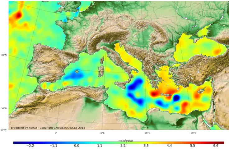
2.3 Regional trends of sea level anomalies in the Mediterranean Sea over 1993-2014 from altimetry-based data. . . 35

(10)

2.4 Tide gauges (yellow dots) and nearest GPS station (blue triangle) used in this study. . . 41 2.5 Temporal availability of satellites in all-sat-merged products. . . 42 2.6 Sample of gridded SLA in the Adriatic Sea. . . 44 3.1 Daily sea level values of the Catania tide gauge. The detected

dis-continuity is indicated by the red line (top panel). The magnitude of the jump has been estimated with the STARS algorithm in order to accurately correct the records (bottom panel) . . . 51 3.2 Mean seasonal cycle of the Valencia tide gauge displayed for a 2-year

period . . . 54 3.3 Mean seasonal cycle of the Genova tide gauge displayed for a 2-year

period . . . 54 3.4 Mean seasonal cycle of the Marina di Ravenna tide gauge displayed

for a 2-year period . . . 55 3.5 Mean seasonal cycle of the Dubrovnik tide gauge displayed for a

2-year period . . . 55 3.6 Mean seasonal cycle of the Siros tide gauge displayed for a 2-year

period . . . 56 3.7 Mean seasonal cycle of the Alexandroupolis tide gauge displayed for

a 2-year period . . . 56 3.8 GPS daily vertical coordinate time series of the MARS (Marseille)

station . . . 66 4.1 Map of SSH change in the Ionian Sea from satellite altimetry data,

over the time interval 1992-2008 . . . 79 4.2 Sea-level trends computed from tide gauge and satellite data along

the Spanish, French and Italian Western coasts . . . 80 4.3 Sea-level trends computed from the tide gauge and the satellite data

along the Greek coasts . . . 82 4.4 Sea-level trends computed from tide gauge and satellite data in the

Adriatic Sea . . . 85 4.5 Sea-level trends computed from VLM-corrected tide gauge, CCI and

AVISO data sets over the period 1993-2013 . . . 89 4.6 Sea-level trends computed from tide gauge, CCI and AVISO data,

(11)

LIST OF FIGURES v 4.7 Differences of the trends computed from AVISO and CCI satellite

data in the Mediterranean Sea, over the period 1993-2013 . . . 91 4.8 Differences of the trends computed from AVISO and CCI satellite

(12)

(13)

List of Tables

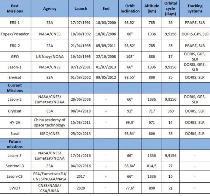
1.1 Summary of Satellite radar altimetry missions. . . 19 1.2 Global mean sea level budget over different time intervals from

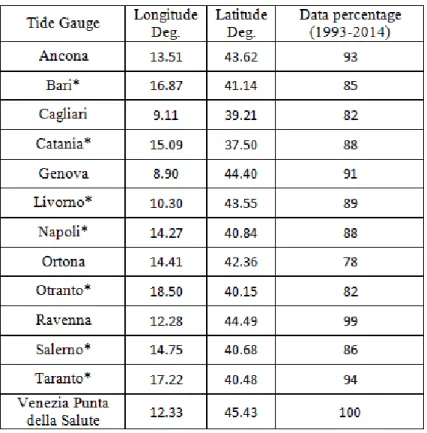
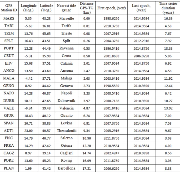
ob-servations and from model-based contributions. . . 27 2.1 Tide gauge stations belonging to the PSMSL used in this work. . . 37 2.2 Tide gauge stations from the RMN. . . 38 2.3 GPS stations used in the analysis. . . 40 2.4 Distances between the tide gauge locations and the satellite SLA

gridded data over the Mediterranean Sea. . . 45 3.1 List of the discontinuities identified in the sea level time series

ob-tained from the RMN network . . . 52 3.2 Mean sea level trends over the period 1993-2014, obtained from tide

gauge data in the Eastern Mediterranean Sea . . . 58 3.3 Mean sea level trends over the period 1993-2014, obtained from tide

gauge data in the Western Mediterranean Sea . . . 59 3.4 Mean sea level trends over the period 1993-2014, obtained from tide

gauge data in the Adriatic Sea . . . 60 3.5 Effect of temporal autocorrelation of the de-trended time series on

standard errors . . . 61 3.6 Average of the standard errors calculated with linear regression and

with autoregressive process of first order . . . 62 3.7 Eastern Mediterranean Sea: trends estimated over the period

1993-2014. The data are the de-seasoned tide gauge data, with IB cor-rection applied . . . 62 3.8 Western Mediterranean Sea: trends estimated over the period

1993-2014. The data are the de-seasoned tide gauge data, with IB cor-rection applied . . . 63

(14)

3.9 Adriatic Sea: trends estimated over the period 1993-2014. The data are the de-seasoned tide gauge data, with IB correction applied . . 64 3.10 Discontinuities detected in the GPS daily vertical coordinate time

series . . . 67 3.11 Trends of VLM estimated with linear regression . . . 68 3.12 Mean sea-level trends derived from monthly de-seasoned satellite

altimetry data over the Eastern Mediterranean Sea . . . 69 3.13 Mean sea-level trends derived from monthly de-seasoned satellite

altimetry data over the Western Mediterranean Sea . . . 70 3.14 Mean sea-level trends derived from monthly de-seasoned satellite

altimetry data over the Adriatic Sea . . . 71 4.1 Eastern Mediterranean Sea: mean sea level trends, estimated over

the period 1993-2014, and VLMs . . . 74 4.2 Western Mediterranean Sea: mean sea level trends, estimated over

the period 1993-2014, and VLMs. . . 75 4.3 Adriatic Sea: mean sea level trends, estimated over the period

1993-2014, and VLMs. . . 76 4.4 Sea-level trends over the period 1993-2013, computed from

GPS-corrected tide gauge, CCI and AVISO data sets . . . 87 4.5 Sea-level trends over the period 1993-2013, computed from tide

(15)

Chapter 1 Sea level rise observations and

causes

The Fifth Assessment Report (AR5) of the Intergovernmental Panel on Climate Change (IPCC) [2013] has established that the warming of the climate system is unequivocal, and, furthermore, that anthropogenic activities are contributing to the climate change. The impacts of global warming have become a question of growing interest in the scientific community, and ongoing discussions on which policies might be effective in response to the climate variations are taking place. Global warming has already given rise to several visible consequences, in particular the increase of the ocean temperature and heat content [Antonov et al., 2005; Levitus et al., 2012], and of melting of glaciers [Gardner et al., 2013], and ice mass from the Greenland and Antarctica ice sheets [Shepherd et al., 2012].

One of the key indicators of climate change is the sea level. Ocean warming causes thermal expansion of sea waters, hence sea level rise. Similarly, water from land ice melt ultimately reaches the oceans, thus also causing sea level rise. Direct sea level observations available since the mid-to-late nineteenth century from in situ tide gauges and, since the early 1990s, from high-precision altimeter satellites, indeed, show that sea level is rising [Nerem et al., 2010; Church and White, 2011], with potentially negative impacts in many low-lying regions of the world.

Coastal zones have changed profoundly during the 20th century with growing populations and economies. Today, many of the world’s megacities are situated on the coast; however, coastal developments have generally occurred with little regard to the consequences of rising sea levels. It is estimated that almost 10% of the world population is living in low-lying coastal zones, thus, sea level rise is generally considered as a major threat of climate change [McGranahan et al.,

(16)

2007]. During the twentieth century, shoreline erosion has been observed in many area of the world [Bird, 1987], however, it remains unclear whether this is due to climate-related sea level rise [Vellinga and Leatherman, 1989] or to more local non-climatic factors such as ground subsidence, coastal management, waves and currents, deficit in sediment supply, etc., [Bird, 1996]. Nevertheless, it is virtually certain that in the coming decades, the expected acceleration of sea level rise, in response to continuing global warming, will intensify the vulnerability of many low-lying, densely populated coastal regions of the world [Wong et al., 2013]. An improved understanding of sea level rise and variability is required in order to reduce the uncertainties associated with future projections, and hence contribute to a more effective coastal planning and management.

1.1 Past sea level estimations

The Earth’s climate has changed throughout history, thereby sea level has changed and continues to change on all time scales. Palaeoclimate information facilitates understanding of Earth system feedbacks on time scales longer than a few centuries, which cannot be evaluated from short instrumental records. Past climate changes also document transitions between different climate states, against which the recent changes can be compared to assess whether or not they are unusual. On time scales between a few thousand to several hundred thousand years, sea level variability responds to an orbital forcing, which denote variations in the Earth’s orbital parameters as well as changes in its axial tilt. Orbital forcing is considered responsible of the transitions between glacial and interglacial periods [Lisiecki, 2010; Huybers, 2011].

Over the glacial cycles sea level can oscillate by more than 100 m as the great ice sheets waxed and waned. These changes in sea level, and the related global average temperature changes, are a direct response to changes in the solar radiation reaching the Earth’s surface; in turn, these solar radiation variations are due to alteration of the Earth’s orbit around the sun. Also, feedbacks processes associated with the related changes in the Earth’s albedo and greenhouse gas concentrations amplify the initial solar radiation changes [Masson-Delmotte et al., 2013]. The relations between sea level, C02 concentration, sea surface temperature and orbital

(17)

1.1. PAST SEA LEVEL ESTIMATIONS 3

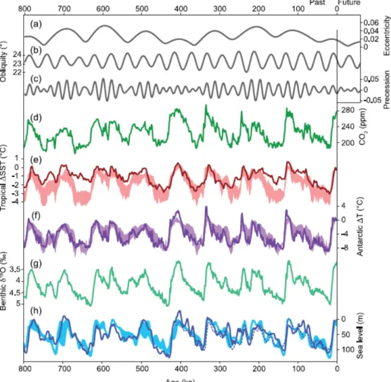
Figure 1.1: Orbital parameters and proxy records over the past 800,000 yr. (a) Eccentricity. (b) Obliquity. (c) Precessional parameter [Berger and Loutre, 1991]. (d) Atmospheric concentration of CO2 from Antarctic ice cores [Petit et al., 1999;

Siegenthaler et al., 2005; Ahn and Brook, 2008; L¨uthi et al., 2008]. (e) Tropical sea surface temperature stack [Herbert et al., 2010]. (f ) Antarctic temperature stack based on up to seven different ice cores [Petit et al., 1999; Blunier and Brook, 2001; Watanabe et al., 2003; European Project for Ice Coring in Antarctica (EPICA) Community Members, 2006; Jouzel et al., 2007; Stenni et al., 2011]. (g) Stack of benthic δ18_{O, a proxy for global ice volume and deep-ocean temperature [Lisiecki}

and Raymo, 2005]. (h) Reconstructed sea level [dashed line: Rohling et al., 2010; solid line: Elderfield et al., 2012]. Lines represent orbital forcing and proxy records, shaded areas represent the range of simulations with climate models [Grid Enabled Integrated Earth System Model-1, GENIE-1, Holden et al., 2010a; Bern3D, Ritz et al., 2011], climate–ice sheet models of intermediate complexity [CLIMate and Bio-sphERe model, CLIMBER-2, Ganopolski and Calov, 2011] and an ice sheet model [Ice sheet model for Integrated Earth system studies, IcIES, Abe-Ouchi et al., 2007] forced by variations of the orbital parameters and the atmospheric concentrations of the major greenhouse gases [From Masson-Delmotte et al., 2013].

(18)

Ice ages are characterized by a low average level of the oceans, up to 130 m below the current level during the last glacial maximum happened around 21,000 years ago [Lambeck et al., 2014]. On the contrary, interglacial periods are marked by high sea level. During the last interglacial (between 116,000 and 129,000 years ago) some palaeodata suggest rates of sea level rise perhaps as high as 1.6 ± 0.8 m/century [Rohling et al., 2008] and sea level about 4–6m above present-day values [Masson-Delmotte et al., 2013] (Fig 1.2).

Figure 1.2: Sea level over the last 500,000 years. This sea level estimate is based on carbonate δ18_{O measurements in the central Red Sea [From Rohling et al., 2008].}

From its level at the last glacial maximum until the beginning of the Holocene, the current interglacial period that began 11,700 years ago, the sea level has risen at an average rate of about 12 mm/yr [Alley et al., 2005; Lambeck et al., 2014]. From about 6,000 to 2,000 years ago, sea level rose more slowly, and during the last 2,000 years the mean sea level has remained quasi stable with a rate of sea level change that did not exceed 0.5 mm/yr [Lambeck et al., 2014], until a recent acceleration since the end of the Nineteenth century, clearly detected in the oldest instrumental observations from tide gauges [W¨oppelmann et al., 2008]. All these past evolutions have been reconstructed from palaeoclimate and geological data. The isotopic composition (ratio 018_/016_{in foraminifera and corals) allows}

estimat-ing the volumes of ice sheets and ocean temperatures to deduce the sea level [Erez, 1978].

(19)

1.2. TIDE GAUGES 5

1.2 Tide Gauges

For the twentieth century and the last decade, two main techniques of sea level observation exist: tide gauges and satellite radar altimetry. Tide gauges measure sea level relatively to the ground, hence data are directly affected by corresponding ground motions. If one is interested in the climate-related components of sea level rise, vertical land motions need to be removed. On the other hand, for studying coastal impacts of sea level rise, it is the relative (including vertical land motion as measured by tide gauges) sea level rise that is of interest. Satellite radar altimetry, unlike tide gauges, measures sea level relative to a geodetic reference frame and thus are not affected by vertical land motion. Data derived from tide gauges are geographically limited while altimeter-measured sea level is characterized by global coverage.

The earliest extended sea level measurements were made in Europe during the eighteenth century. These data were visual observations of the heights and times of high and low waters. Many entrances to docks were equipped with what were then called “tide gauges”, graduated markings on their stone walls to indicate water depth over the dock sill. Visual measurements could have had centimeter-level accuracy in calm weather conditions, but would have been much less accurate in the presence of waves [Woodworth et al., 2011].

A more accurate measurement of sea level is possible since the 1830s thanks to automatic tide gauges, capable of recording the full tidal curve, not just the high and low waters. These instruments employed a tube, known as a stilling well, with a float connected to a wire, running over pulleys to a pen moving up and down as the tide rose and fell, thereby drawing a tidal curve on a rotating drum of paper. New technologies have since replaced float gauges at many locations such as radar gauges, which emit a radar signal towards the sea surface and measure the travel time of the reflected signal in order to deduce water level. However, it is important to note that float gauges have provided the bulk of the historical sea level data set, and they still constitute a large fraction of the global network. In order to measure long-term sea-level changes accurately, tide gauge observations must be compared to a well-defined fixed level or datum. Benchmarks are commonly used for this purpose as they are located on a stable surface to provide a local height reference level. The stability of a particular benchmark cannot be guaranteed, thus, it is good practice to measure the elevation of the tide gauge benchmark relative to a group of other local benchmarks, and to check them periodically to ensure that they maintain, or not, these elevations relative to one another (Fig

(20)

1.3).

Figure 1.3: Schematic diagram showing the tide gauge connections to SLR/VLBI reference system [From Zerbini et al., 1996].

Tide gauge data have some limitations. First of all, they have a heteroge-neous spatial distribution. The Permanent Service for Mean Sea Level [PSMSL; Woodworth and Player, 2003] is the largest global data bank, about 2000 stations, for long term tide gauge sea level observations concerning the twentieth century. Figure 1.4 presents an overview of the data holdings. There are much greater con-tributions from the Northern Hemisphere and from the second half of the twentieth century. This bias should always be kept in mind when calculating global mean sea level rise.

Another major difficulty is that tide gauge records are relative to the local land, thus they measure the combined effect of ocean volume change and vertical land motion (VLM). In active tectonic and volcanic regions, or in areas subject to strong ground subsidence due to natural causes (for examples, sediment loading in river deltas) or human activities (groundwater and hydrocarbons extraction), tide gauge data are directly affected by relevant ground motions. One component of the VLM is the post-glacial rebound, the viscoelastic response of the Earth crust and mantle to last deglaciation (nowadays called glacial isostatic adjustment, GIA). The problem of correcting the tide gauge records for the VLM has only been partially solved. Most studies of twentieth century time series are only accounting for the GIA [Douglas, 1991, 1997; Church and White, 2011], since this is the only vertical motion that can be described globally by a physical model. Land motions due to GIA are described by global geodynamic models of the Earth continued

(21)

1.2. TIDE GAUGES 7

Figure 1.4: Overview of PSMSL tide gauge database. (a)Stations represented in the data set of the Permanent Service for Mean Sea Level (PSMSL). (b)Stations with long records containing more than 60 years of data [From Woodworth et al., 2011].

response to deglaciation [Peltier, 2001, 2004]. However, in some areas, VLM due to tectonic activity, groundwater mining, or ground fluids exploitation is larger than GIA and can affect the estimate of reliable sea-level rates [King et al., 2012; Wöppelmann et al., 2013]. An alternative approach is the use of space geodetic techniques to measure directly VLM and to correct the tide gauge data [Zerbini et al., 1996; Bouin and Wöppelmann, 2010]. More recently, Global Positioning System (GPS) receivers have been installed at tide gauge sites to measure VLM. However, these VLM measurements are only available since mid-late 1990s at the earliest, and could only be extrapolated into the past, if the assumption of a constant trend can be made. Additionally, at present the GPS installations do not cover all tide gauge sites [Santamar`ıa-Gòmez et al., 2012]. The information on VLM provided by GPS at tide gauges is the approach used in this study, and will be discussed in more detail in the following chapter.

(22)

1.3 Satellite Radar Altimetry

Since the early 1990s, sea level is routinely measured with quasi-global coverage and a few days/weeks revisit time (called “orbital cycle”) by altimeter satellites. Compared to tide gauges, which provide sea level relative to the Earth crust, satellite altimetry measures sea level variations relative to the center of mass of the Earth. As a result, satellite altimetry measurements of sea level are made in an absolute reference system and do not need to be corrected for VLM.

1.3.1 Basic principle

The concept of the satellite altimetry measurement is simple [Chelton et al., 2001]: the onboard radar altimeter transmits microwave radiation toward the sea surface and is partly reflected back to the satellite. The signal two-way travel time is measured and the satellite distance from the sea surface can then be estimated. Figure 1.5 presents a schematic diagram of how satellite radar altimetry works.

Figure 1.5: Altimetry principle: Altimeters emit signals toward the Earth, and receive the echo from the sea surface, after the reflection. The sea surface height is obtained by the difference between the satellite’s position relative to the reference ellipsoid and the satellite distance from the sea surface (range) (From AVISO).

(23)

1.3. SATELLITE RADAR ALTIMETRY 9 Radar altimeters permanently transmit signals at high frequency (over 1700 pulses per second) toward the Earth, and receive the echoes from the sea surface. The signal round-trip time between the satellite and the sea surface is deduced by analyzing the echo waveform. This is the curve describing the power of the signal reflected back to the altimeter. The electromagnetic radiation transmitted by the satellite is attenuated while going through the atmosphere and finally the pulse leading edge hits the water surface. As the incident pulse strikes the surface, it illuminates a circular region increasing linearly with time. After the pulse trailing edge has intersected the surface, it remains constant. At this moment, the return waveform has reached its peak. Travelling back to the satellite, the signal power is further attenuated by both the atmosphere and because the reflected signal no longer comes from directly below (Fig 1.6, left panel).

Figure 1.6: Pulses reflection over a flat (left) and rough sea (right) (adapted from AVISO).

This description is what happens over an ideal flat ocean, such standard wave-form is also named “Brown Model” [Brown, 1977]. Surfaces characterized by sig-nificant slopes, such as those present in rough seas, make accurate interpretation more difficult. In this case, the pulse strikes the crest of one wave and of a series of other crests, causing the reflected wave amplitude to increase more gradually compared to the case of the flat ocean (Fig 1.6, right panel). From the change in slope of the waveform leading edge, the Significant Wave Height (SWH) can be estimated. The SWH is defined to be the average crest-to-trough height of the 1/3 highest waves and is usually denoted as H1/3. The power of the return signal is also

related to the sea surface roughness which is highly correlated with near-surface winds, thus, wind speed can be estimated from empirical formulae relating it to the signal backscattered power [Chelton and McCabe, 1985]. The return time is defined as the moment in which the mid-point of the waveform leading edge is detected (Fig 1.7).

(24)

Figure 1.7: Basic waveform shape. Several parameters can be deduced: epoch at mid-height gives the time the radar pulse took to travel the satellite-surface distance and back again; P is the energy of the pulse which can be used to calculate the backscatter coefficient; Po is the instrumental noise; the leading edge slope can be related to the significant wave height (SWH); the skewness is the leading edge curvature; the trailing edge slope is linked to any mispointing of the radar antenna (i.e. any deviation from nadir of the radar pointing) (from AVISO).

The time measurement, scaled by the speed of light in the vacuum, yields a range measurement:

R = ct

2 (1.1)

The travel time needs to be known very accurately (a precision of 30 ps is required to achieve an accuracy of 1 cm on the height), so the actual measurements are formed by averaging a large number of individual radar echoes. These final obser-vations, called the Geophysical Data Records (GDRs), are the data which will be further processed. Once the range has been calculated, the quantity of scientific interest can be computed, namely the sea surface height (SSH), that is the sea surface above a reference ellipsoid:

SSH = S–R (1.2) where S is the satellite altitude above the reference ellipsoid and R is the range. Thus, the ability to determine with high accuracy the satellite orbit is a key factor in satellite altimetry, since any error in the satellite orbit radial component will directly affect the SSH measurement. Precise orbits are provided by the space agencies.

(25)

1.3. SATELLITE RADAR ALTIMETRY 11

1.3.2 Corrections of altimeter measurements

Several sources of error affect the altimeter measurements. They can be grouped in four different categories:

• instrumental errors; • satellite position errors; • signal propagation errors; • geophysical errors.

1.3.2.1 Instrumental errors

To obtain accurate range measurements, the measured two-way travel time must be corrected for a number of instrumental errors (for detailed information, see Chelton et al., 1989, 2001). Under instrumental errors we can identify: the Doppler shift effect, caused by a change in the frequency of the returned signal due to the relative velocity between the satellite and the sea surface; the effect of accelerations of the spacecraft relative to the sea surface; the oscillator drift; altimeter calibration and pointing angle errors. The last one is the largest, resulting in a 2 cm range error for a 0.2◦ off-nadir pointing. Some of these errors can be evaluated on the ground before launch, and some during the initial mission calibration phase.

1.3.2.2 Satellite position errors

Many efforts have been made since the beginning of the satellite altimetry era to develop techniques capable of minimizing the orbit errors, since high preci-sion is required for oceanographic applications [Tapley et al., 1994; Le Traon and Ogor, 1998; Rudenko et al., 2012; Couhert et al., 2015]. Precise Orbit determi-nation (POD) is the procedure allowing estimating the three-dimensional position of the satellite center-of-mass, at regularly spaced time intervals, in a well-defined reference frame. POD combines accurate and complex mathematical models, de-scribing the dynamics of the satellite motion with high precision observations of the satellite position [Tapley et al., 2000]. The motion of a close Earth satellite is perturbed by a number of forces which are, in relative order of importance:

• Earth gravity field including solid Earth and ocean tides; • gravity perturbations due to the Moon, Sun and major planets;

(26)

• direct solar and Earth albedo radiation pressure; • atmospheric drag;

Uncertainties in modeling the Earth gravity field have long been the main source of orbit error in POD. Gravity force models have greatly improved since the beginning of the altimetry era, thanks to dedicated gravity missions like GRACE (Gravity Recovery and Climate Experiment) and the more recent GOCE (Grav-ity Field and Steady-State Ocean Circulation Explorer), launched in March 2002 and March 2009, respectively [Pavlis et al., 2008; Mayer-G¨urr et al., 2012]. The current models for the various gravitational effects are well documented in the International Earth Rotation Service (IERS) Conventions [IERS, 2010]. Non-gravitational forces such as solar radiation pressure and atmospheric drag, depend on the size and shape of the spacecraft, thus their modeling is easier for satellites with a simple geometry.

Radar altimetry measurements cannot provide an accurate determination of the satellite orbit, thus, independent observations of the satellite motion are re-quired. Three main types of tracking techniques are employed to acquire these observations, each with different measurement characteristics, temporal and geo-graphic coverage. Most recent altimetry satellites can be tracked by means of, at least, two techniques. Usually, a laser retroreflector array onboard the spacecraft, or just a few corner cube retroreflectors, support tracking by the satellite laser ranging (SLR) technique. Other systems include Doppler Orbitography and Ra-diopositioning Integrated by Satellite (DORIS) and the Global Positioning System (GPS).

1.3.2.3 Signal propagation errors

We can distinguish two main sources of error: the atmospheric refraction delay and the sea-state bias.

Atmospheric refraction

The effects of atmospheric refraction are generally expressed in terms of path delay. The presence of the atmosphere delayed the propagation of the altimeter signal, increasing the measured two-way travel time, which differs from the esti-mate assuming the free-space value for the speed of light. Failure to correct for atmospheric refraction results in a range estimate that is longer than the true range. Ionospheric and tropospheric refraction errors are considered separately; in

(27)

1.3. SATELLITE RADAR ALTIMETRY 13 turn, tropospheric error can be broken down into dry and wet tropospheric delay. Ionospheric refraction

Ionospheric refraction of altimetric radar signals is due to the dielectric proper-ties of the upper atmosphere associated with the presence of free electrons. These are produced by the ionization, in the high atmosphere, of the incident solar ra-diation. The effective light speed is reduced by an amount depending on the Total Electron Content (TEC) and on the wavelength of the radar signal [Calla-han, 1984]. The range delay is estimated from models of the vertically integrated electron density. However, the TEC is mainly correlated with the geomagnetic field, therefore is characterized by significant spatial variations. The TEC is also correlated with the solar activity and thus present strong diurnal and seasonal variability. Therefore, given that the delay depends on the signal wavelength, it can be estimated using a dual frequency altimeter. The information obtained from different frequencies allows estimating a reliable delay correction [Imel, 1994]. Dry tropospheric refraction

The dry component of atmospheric refraction is, by far, the largest correction that need to be applied to altimeter measurements. The mass of dry air molecules in the atmosphere causes an overestimation of the measured range of about 2.3 m. The correction is directly proportional to the atmospheric pressure measured at sea level and, in units of centimeters, can be approximated by [Chelton et al., 2001]:

∆SSHdry ≈ 0.2277P0(1 + 0.0026 cos 2ϕ) (1.3)

where P0 is the sea level pressure expressed in mbar and ϕ is the latitude of the

measured sea surface point. Wet tropospheric refraction

The wet tropospheric correction includes both the water vapor and the cloud liquid water droplet contributions to atmospheric refraction. The water content in the troposphere is highly variable in space and time, causing path delays ranging from 5 cm to 30 cm, according to the elevation angle of the observation. The wet tropospheric correction is computed using both on-board microwave radiometer measurements [Keihm et al., 1995], and atmospheric models of water vapor content [Fernandes et al., 2010, 2014].

(28)

Sea-state bias

The effect of the actual sea state on the reflected signal is referred as the sea-state bias (SSB). The size of the reflecting area depends on the roughness of the sea surface. At wave troughs the reflection is higher than at wave crests. Systematic corrections are required because the sea surface height measured by the altimeter is biased toward wave troughs. The SSB correction ε can be expressed as a percentage of the SWH [Tran et al., 2010]:

ε ≈ β · SW H (1.4) where β is between 1 and 5%. More accurate SSB corrections are obtained us-ing empirical models derived from SWH and wind speed observations and from numerical ocean wave models [Tran et al., 2010].

1.3.2.4 Geophysical errors

A satellite radar altimeter measures the instantaneous sea surface height that is affected by time-dependent geophysical effects, including solid earth and ocean tides, polar tide, ocean loading and high and low frequency sea surface response to atmospheric pressure and wind stress. By removing these effects time independent SSHs are obtained.

Ocean tides and ocean loading corrections

Ocean tides are periodic deformations of sea surface resulting from gravita-tional attraction of celestial bodies, in particular, the Moon and the Sun. The relative movements of the Moon and the Sun with respect to the Earth, combined with the Earth own rotation, result in periodic displacements of water masses with different order of magnitude. In open ocean, tide amplitudes are typically 1-2 m, while they can reach several meters in coastal regions [Le Provost, 2001]. The most recent models use assimilated altimeter data as constraints and estimate tides globally with high spatial resolution [Ray et al., 2013]. Ocean tides also cause oceanic mass redistribution with associated load change on the crust, therefore, producing time-varying deformations of the Earth. The ocean tidal loading effect is computed from ocean tide models [Ray, 1998].

Solid Earth tide correction

(29)

1.3. SATELLITE RADAR ALTIMETRY 15 including the ocean bottom, due to luni-solar forcing. Solid Earth tides occur at the same frequencies as the ocean tides with amplitudes of about 50 cm. The solid Earth tide correction can be derived from tide-generating potential models depend-ing upon Love numbers assumdepend-ing an elastic Earth with uniform mass [Cartwright and Tayler, 1971; Cartwright and Edden, 1973].

Polar tide correction

The pole tide is a tide-like motion of the ocean surface, resulting from small effects due to the variation of the Earth rotation axis. These perturbations primar-ily occur at annual period, and at a 433-day period called the Chandler wobble, with amplitudes of about 2 cm. The pole tide correction is provided by models which require knowledge of the pole position [Wahr, 1985; Desai, 2002].

Atmospheric pressure and wind forcing correction

The Inverse Barometer (IB) is a correction accounting for variations in sea surface height due to atmospheric pressure variations (atmospheric loading). The ocean responds directly to atmospheric pressure changes: sea level rises (falls) in connection with low (high) pressure systems. The inverse barometer correction assumes an instantaneous static local response of the sea level to pressure varia-tions, so that the total pressure at the ocean bottom is constant. The correction is expressed by the following equation [Dorandeu and Le Traon, 1999]:

IB = −0.9948(P − PRef) (1.5)

where P is the instantaneous local sea level pressure in millibar and PRef is the time

varying mean global surface atmospheric pressure over the oceans in millibar. In many applications, PRef is assumed to be constant, equal to 1013.3 mbar. The scale

factor of -0.9948 implies that a local increase of 1 mbar in atmospheric pressure locally depresses the sea surface by about 1 cm. More precise corrections can be calculated using meteorological models. The ocean response to meteorological forcing is not completely accounted for by simply applying the inverse barometer correction [Wunsch and Stammer, 1997]. The classic IB formulation identifies the static response of the ocean to atmospheric pressure forcing, while wind effects are totally ignored [Carrere and Lyard, 2003]. Several studies have pointed out that the ocean has a clear dynamic response to pressure forcing at high frequencies (periods below 3 days) and at high latitudes, and that wind effects prevail around the 10 days period [Fukumori et al., 1998; Ponte and Gaspar, 1999]. Therefore,

(30)

this high frequency variability is corrected by using independent ocean models. At present, the effect due to atmospheric pressure and wind forcing are combined in the so called Dynamic Atmospheric Correction (DAC) [Carrere and Lyard, 2003; Carrere et al., 2015].

1.3.3 Sea Level Anomalies

With the introduction of the models described above, the expression for the measured sea surface height can be rewritten in a more complete form as follows: SSH = Scor− (R + hi+ hiono+ hdry+ hwet+ hssb+ hotide+ hol+ hstide+ hptide+ hdac)

(1.6) where Scor is the satellite altitude corrected for orbit errors, R is the

instanta-neous distance between the altimeter antenna and ocean surface. The following corrections represent hi the sum of the instrumental errors, hiono the ionospheric

delay, hdry the dry tropospheric component, hwetthe wet tropospheric component,

hssb the sea-state bias, hotide the ocean tide, hol the ocean loading, hstide the solid

Earth tide, hptide the pole tide and hdac the dynamic atmospheric effect,

respec-tively. The SSH obtained in this way is time-independent and is the sum of three remaining components. They are the height of the geoid above the reference ellip-soid, and both a permanent and a variable part of the ocean dynamic topography. The geoid is an equipotential surface of the Earth gravity field and can be defined as the static part of the sea surface. In absence of other forcings, the sea surface would be a surface of constant gravity potential corresponding to the marine geoid. Because the gravity field varies geographically, the geoid is an undulated surface and is, generally, described in terms of geoid undulations N, that is the heights of the geoid with respect to the reference ellipsoid. Geoid undulations are in the order of ± 100 m. The highest negative values, -106 m, are found in the Indian Ocean, whereas the highest positive values are encountered over Indonesia (+85 m) and in the Northern Atlantic Ocean (+61 m) [Limpach, 2010]. A schematic diagram of the effect of a bump and a depression at the ocean floor on the sea surface is shown in Figure 1.8.

(31)

Figure 1.8: Schematic diagram of a bump and a depression at the ocean bottom and the corresponding marine geoid. Vectors indicate the gravitational acceleration along the geoid [From Limpach, 2010].

The ocean topography can be divided into a quasi-stationary part called the mean dynamic topography (MDT), with amplitude of magnitude of about 1 m, and a time-variable component due to change in the ocean circulation, the amplitude of which is in order of a few decimeters (Fig 1.9). The sum of the permanent and the variable part is known as the absolute dynamic topography (ADT) which is the sea surface height relative to the geoid, and is represented by the following equation:

SSH = N + ADT (1.7) The time variable part of the SSH is used in oceanographic studies. The Sea

Figure 1.9: Altimetry heights naming convention. (from AVISO).

Level Anomaly SLA, computed by subtracting from the SSH a temporal reference hSSHi is defined as follows:

(32)

This temporal reference can be both a Mean Profile (MP) and a gridded Mean Sea Surface (MSS). The MSS represents the ocean surface averaged over an appropriate time period in order to remove annual, semi-annual, seasonal and spurious sea surface height signals [Picot et al., 2003]. The MSS corresponds to the sum of the geoid undulation N and of the mean dynamic topography MDT, over a selected time period, and it is referred to a given ellipsoid [Hernandez and Schaeffer, 2001].

1.3.4 Satellite altimetry missions

The development of accurate satellite altimeter systems started in the early 1970s and made possible the first nearly global observations of sea level. These early altimeters were intended to demonstrate proof of the concept of radar altime-try. However, till the launch of TOPEX/Poseidon (T/P), on August 10 1992, these measurements were severely affected by the inadequate knowledge of the Earth gravity field, contributing to a poor determination of the orbits of the altimetry satellites. This joint NASA/CNES (the USA and the French space agencies, re-spectively) was launched with the main objective of observing and understanding ocean circulation. Numerous improvements were made to Topex/Poseidon com-pared to previous altimetry systems. This included a specially-designed satellite, a suite of sensors, satellite tracking systems and orbit configuration, as well as the development of an optimal gravity field model for precision orbit determination, and a dedicated ground system for mission operations. Follow-on missions are those of the Jason series, which have inherited the T/P main features, although technological improvements constantly contribute to upgrading these satellites. Satellite altimetry has become an operational technique, therefore the availability of these observations is guaranteed for the future. Table 1.1 presents, starting from 1990s, the history, perspective and characteristics of satellite altimetry missions.

(33)

(34)

1.4 Causes and Observations of current GMSL

1.4.1 Main factors of current global mean sea level rise

The main factors causing current GMSL rise are the thermal expansion of sea waters, land ice loss, and fresh water mass exchange between oceans and land water reservoirs (Fig 1.10); these different components have been the subject of many studies [Antonov et al., 2005; Rignot et al., 2011; Shepherd et al., 2012; Wada 2012]. These contributions vary in response to natural climate variability and global climate change [Rhein et al., 2013].

Figure 1.10: Schematic of climate-sensitive processes and components that can influence global and regional sea level. Changes in any one of the components or processes shown will result in a sea level change [From Cazenave and Le Cozannet, 2014].

The oceans are a central component of the climate system, by storing and transporting large amounts of heat. Indeed, more than 90% of the heat absorbed by the Earth over the last 50 years due to global warming is stored in the ocean [Levitus et al.,2012]. As the oceans warm, they expand and sea level rises, re-sulting in changes of the ocean water density (steric effect). It is estimated that for a 1000 m column of sea water the expansion is about 1 or 2 cm for every 0.1◦C of temperature increase [Church et al., 2010]. Density changes induced by temperature changes are called thermosteric, while density changes induced by salinity changes are called halosteric. Both are important for regional sea-level changes [Durack and Wijffels, 2010]; however only the thermosteric contribution is significant for the global average ocean volume change. Thermosteric sea level

(35)

1.4. CAUSES AND OBSERVATIONS OF CURRENT GMSL 21 rise was a major contributor to 20th century sea level rise, and is projected to continue during the 21st century and for centuries into the future [Rhein et al., 2013]. Ocean thermal expansion has been estimated from analyses of Expand-able Bathy Thermographers (XBT) data collected over the past 50 years by ships [Ishii and Kimoto, 2009; Levitus et al., 2012], and during the last 10 years by automatic profiling floats of the Argo system, mostly in the upper layers (up to depths of 700-2000 m). These data indicate that the ocean heat content has in-creased during the past few decades, in particular, since 1970 [Ishii and Kimoto, 2009; Levitus et al., 2012], resulting in a significant thermosteric sea level rise (Fig 1.11). Although very sparse, the few available deep ocean temperature measure-ments (below 2000 m) indicate that the deep ocean has also warmed [Purkey and Johnson, 2010] in the recent decades, but its exact contribution to sea level rise remains uncertain. In addition, to the much improved observational database, data assimilation techniques combining observations and models are now being applied to the ocean. This approach helps overcoming the inadequate data dis-tribution and allows synthesizing all available data in one consistent estimate of the evolving ocean [Gregory et al., 2001]. Since the 1960s and 1970s, global ocean and coupled atmosphere-ocean general circulation models (AOGCMs) have been developed, and they improved rapidly as numerical techniques and ocean data sets increased. These models are the basis for the projections of global averaged steric sea level rise and the regional distribution of sea level rise during the 21st century and beyond [Gregory et al., 2006, 2013].

(36)

Figure 1.11: Time series of halosteric (red curve), thermosteric (black curve) and total steric sea level component (mm) for the 0-700 m (top) and 0-2000 m (bot-tom) layers based on running pentadal (five-year) analyses. Reference period is 1955-2015. Each pentadal estimate is plotted at the midpoint of the 5-year period [updated from Antonov et al., 2005, NOAA 2015].

(37)

1.4. CAUSES AND OBSERVATIONS OF CURRENT GMSL 23 The other main contribution to sea level rise is provided by the increase of water mass due to melting of mountain glaciers and ice sheets from Greenland and Antarctica. GMSL change resulting from ocean mass variation is called barystatic. A signal of added mass to the ocean propagates around the globe such that all regions experience a sea level change [Lorbacher et al., 2012]. In addition, an influx of freshwater changes ocean temperature and salinity, and thus, changes ocean currents and local sea level [Stammer, 2008]; these signals need decades to propagate around the global ocean. The amount of barystatic sea level change due to the addition or removal of water mass is called sea level equivalent (SLE). This is the conversion of a water mass (ice, liquid or vapor) into a volume, by using a density value equal to 1000 kg m−3 divided by the present day ocean surface equal to 3.625 · 1014_m2_{. Thus, a water mass of 362.5 · 10}12 _{kg need to be added to the}

ocean to cause 1 mm of global mean sea level rise.

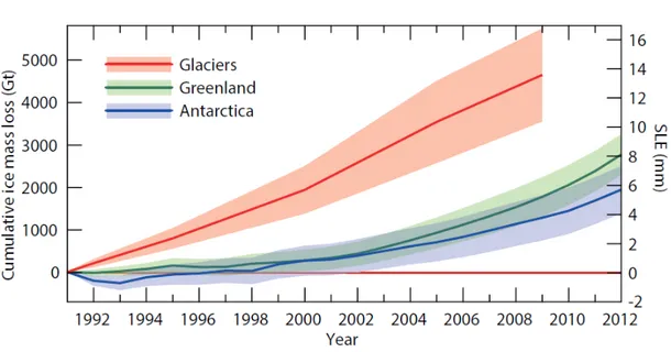
Being very sensitive to global warming, mountain glaciers and small ice caps have retreated worldwide during the twentieth century, with significant accelera-tion since the early 1990s [Meier et al., 2007]. Changes in glaciers are measured through the survey of glacier extension, mass and volume by means of a wide range of observational techniques [Vaughan et al., 2013]. Most glaciers are now monitored using remote sensing methods such as aerial photography and satellite imaging [Leclercq and Oerlemans, 2012], and by GPS observations [King, 2004]. Since 2003, accurate measurement of the Earth gravity field variations from the GRACE satellites provide a most significant contribution in estimating ice mass variation/changes [Gardner et al., 2013]. For the mass balance of ice sheets, little is known before the 1990s because of inadequate and incomplete observations. It is estimated that if totally melted, Greenland and West Antarctica (the instable part of the continent) would raise sea level by about 7 m and 3-5 m, respectively [Lemke et al., 2007]. Even a small amount of ice mass loss from the ice sheets would be able to produce substantial sea level rise; thus, the contribution of the ice sheets to GMSL need to be controlled with higher precision. Since the early 1990s, differ-ent remote sensing observations (airborne and satellite radar and laser altimetry, interferometric synthetic aperture radar –InSAR–, and space gravimetry from the GRACE mission) have provided important observations of the mass balance of the ice sheets, indicating that Greenland and West Antarctica are losing mass with an accelerated rate [Velicogna, 2009; Rignot et al., 2011]. For the period 1993-2003, less than 15% of the rate of global sea level rise was due to the ice sheets [Lemke et al., 2007], but this contribution has nearly doubled since 2003-2004 [Shepherd et al., 2012; Vaughan et al., 2013]. In addition to these observations, Regional

(38)

Figure 1.12: Contribution of Glaciers and Ice Sheets to sea level change. Cumula-tive ice mass loss from glacier and ice sheets (in sea level equivalent) is 1.0 to 1.4 mm/yr for 1993-2009 and 1.2 to 2.2 mm/yr for 2005-2009 [From Vaughan et al., 2013].

Climate Models (RCMs) are now the primary source of ice sheet surface mass balance (SMB) projections. They incorporate, or are coupled to, sophisticated representations of the snow and ice surfaces mass and energy budget [Lenaerts et al., 2012]. SMB is primarily the difference between snow accumulation and ablation (the total melted snow and ice). These models require information on the state of the atmosphere and of the ocean at its boundary. These information are derived from reanalysis data sets or AOGCMs. The main challenge, faced by models attempting to assess sea level change from glaciers, is the small number of glaciers for which mass budget observations are available (about 380) [Cog-ley, 2009a], as compared to the total number (more than 170,000) [Arendt et al., 2012]. Statistical techniques are used to derive relations between observed SMB and climate variables for the small sample of surveyed glaciers, these relations are then used for unsurveyed regions of the world. These techniques often include area-volume scaling to estimate glacier volume from their more readily observable areas [Marzeion et al., 2012; Hirabayashi et al., 2013].

An additional contribution to changing sea level comes from the storage of wa-ter on land: in lakes, dams, rivers, wetlands, soil moisture, snow cover, permafrost, and aquifers. These respond to both climate variations and to anthropogenic ac-tivities (dam building, underground water mining, irrigation, urbanization, defor-estation, etc.). No global data sets exist to estimate the historical land water components; estimates of climate related changes in land water storage over the

(39)

1.4. CAUSES AND OBSERVATIONS OF CURRENT GMSL 25 past few decades rely on global hydrological models [Milly et al., 2010] and, since 2002, on space gravimetry observations from the GRACE mission that allows direct determination of the total land water storage variations due to the combination of climate variability and human activities [Llovel et al., 2011]. Model-based es-timates of land water storage change, caused by natural climate variability, do not suggest any long-term climatic trend during the second half of the twentieth century [Milly et al., 2003; Ngo-Duc et al., 2005]; however, they documented in-terannual to decadal fluctuations, equivalent to several millimeters of sea level. Recent studies have shown that the observed GMSL interannual variability corre-lates with ENSO (El Niño Southern Oscillation) indices [Nerem et al., 2010] and is inversely related to ENSO-driven changes of terrestrial water storage, especially in the tropics [Llovel et al., 2011]. During El Niño events, sea level (and ocean mass) tends to increase [Chambers, 2011; Cazenave et al., 2012]. The reverse hap-pens during La Niña events, as seen during 2010-2011, when there was a decrease in GMSL due to a temporary increase in water storage on the land, especially in Australia, northern South America, and southeast Asia [Boening et al., 2012]. Human interventions on land water storage also induce sea level changes. Chao et al. [2008] showed that dam building along rivers and associated reservoir im-poundments has lowered sea level by about -0.5 mm/yr during the second half of the twentieth century. Inversely, groundwater extraction for crop irrigation in regions of intensive agriculture has led to a few tenths of mm/yr sea level rise [Wada et al., 2013]. Although subject to considerable uncertainty, estimates for the past few decades suggest near cancelation between net groundwater depletion and dam/reservoir contribution [Konikow, 2011; Wada et al., 2012]. However, the situation might change in the future because of expected increasing groundwater depletion and decreasing dam building, leading to a net positive contribution to sea level [Konikow, 2011; Wada et al., 2012, 2013].

1.4.2 Observed sea level rise and budget estimations

Many studies have been published in recent years on the comparison between observed sea level rise and the sum of the estimated single contributions [Church et al., 2011; 2013; Hanna et al. 2013; Dieng et al., 2015]. The observed sea level change from instrumental records is mainly composed of tide gauge measurements over the past two centuries, and, since the early 1990s, of satellite-based radar altimeter measurements.

(40)

gauge records data base [Holgate et al., 2013; PSMSL 2015] is challenging. In fact, tide gauges sample the ocean sparsely and non-uniformly, with a bias towards coastal sites and the Northern Hemisphere, there are a few sites at latitude greater than 60◦, and significant interannual and decadal-scale fluctuations are present in all time series [Church and White, 2011; Hay et al., 2013]. Many authors have compute the mean rate of twentieth century GMSL rise from the available tide gauges data, all with different approaches [Jevrejeva et al., 2006; Holgate, 2007; Jevrejeva et al., 2008; Church and White, 2011]. The estimates of GMSL rise obtained from these studies ranges from 1.6 to 1.9 mm/yr. Also, IPCC AR5 [2013] suggests that there is a 95% probability that GMSL rise from 1901 to 1990 was greater than 1.3 mm/yr. However, independent model and data-based estimates of the individual sources of GMSL, including mass flux from glaciers and ice sheets, thermal expansion of oceans, and changes in land water storage, are insufficient to account for the GMSL rise estimated from tide gauge records [Gregory et al., 2013]. Church et al. [2013] presents a list of contributing effects to GMSL rise from 1901 to 1990 (see Table 1.2), the total budget turns out to be +0.5 ± 0.4 mm/yr (90% Confidence Interval - CI) lower than the tide gauge derived rate of +1.5 ± 0.2 mm/yr (90% CI) estimated by Church and White [2011] for the same period. This discrepancy has been attributed to underestimation of almost all possible sources: thermal expansion, glacier mass balance, and Greenland or Antarctic ice sheet mass balance [Church et al., 2013].

(41)

1.4. CAUSES AND OBSERVATIONS OF CURRENT GMSL 27 Table 1.2: Global mean sea level budget (mm/yr) over different time intervals from observations and from model-based contributions. The modeled thermal expansion and glacier contributions are computed from the CMIP5 (Coupled Model Intercom-parison Project Phase 5 [IPCC AR5, 2013]) results, using the model of Marzeion et al. [2012a] for glaciers. The land water contribution is due to anthropogenic intervention only, not including climate-related fluctuations. Notes: a) data for all glaciers extend to 2009, not 2010; b) This contribution is not included in the total because glaciers in Greenland are included in the observational assessment of the Greenland ice sheet; c) Difference between observed GMSL rise and the sum of the individual components [From Church et al., 2013].

A more recent study performed by Hay et al. [2015] revisits the analysis of GMSL since the start of the twentieth century using two statistical methods: Kalman smoothing (KS) and Gaussian process regression (GPR). Both approaches naturally accommodate spatially sparse and temporally incomplete sampling of a global sea level field, thus providing a rigorous, probabilistic framework for uncer-tainty propagation, correcting also for a distribution of GIA and ocean models (see Hay et al., 2015, for complete description of these methods). The mean GMSL rate for 1901-1990 estimated from the KS and GPR analysis are, respectively, 1.2 ± 0.2 mm/yr and 1.1 ± 0.4 mm/yr, significantly lower than the estimates of other studies for the same period (Fig 1.13). This estimate closes the sea-level budget for 1901-1990 estimated in AR5 [Church et al., 2013] without appealing to an un-derestimation of individual contributions from ocean thermal expansion, glacier melting, or ice sheet mass balance [Hay et al., 2015].

(42)

Figure 1.13: Time series of GMSL for the period 1900-2010. Shown are estimates of GMSL based on KS (blue curve), GPR (black curve), Ref.3 refers to Church and White [2011] (magenta curve) and Ref.4 to Jevrejeva et al., [2008] (red curve). Shaded regions show ±1σ uncertainty. Inset, trends for 1901-1990 and 1993-2010, and accelerations, all with 90% CI (not available for Jevrejeva et al., [2008]). Since the GPR methodology outputs decadal sea level, no trend is estimated for 1993-2010 [From Hay et al., 2015].

Budget studies are more reliable for the satellite altimetry era due to the in-troduction of several global observation systems. In addition to satellite radar altimetry, the GRACE mission, the network of Argo buoys, the InSAR and GPS techniques, made it possible to accurately quantify each budget component (Fig 1.14).

In Church et al., 2013, the observed rate of global mean sea level rise over the 1993-2010 time span is compared to estimates of the sum of individual components. The rate of GMSL rise for this period is +3.2 ± 0.4 mm/yr, based on the average of altimeter time series published by multiple groups [Ablain et al., 2009; Beckley et al., 2010; Nerem et al., 2010; Church and White, 2011; Masters et al., 2012]. The tide gauges analysis from Church and White [2011] for the 1993-2010 period gives a rate of +2.8 ± 0.5 mm/yr. The result of the KS method from Hay et al.

(43)

1.4. CAUSES AND OBSERVATIONS OF CURRENT GMSL 29

Figure 1.14: Global mean sea level from altimetry from 2005 to 2012 (blue line). Ocean mass changes are shown in green (as measured by Gravity Recovery and Climate Experiment (GRACE)) and thermosteric sea level changes (as measured by the Argo Project) are shown in red. The black line shows the sum of the ocean mass and thermosteric contributions [From Church et al., 2013].

[2015] is in agreement with the previous results, providing a rate of +3.0 ± 0.7 mm/yr. The different analysis show that the rate of sea level rise during the last two decades is about twice as much the mean rise of the twentieth century. Hay et al. [2015] calculate an acceleration of 0.009 ± 0.002 mm/yr2 _{based on the Church}

and White [2011] time series, but, using the GMSL rate calculated with the KS method (1.2 ± 0.2 mm/yr for the period 1900-1990) the estimated acceleration is significantly higher and equal to 0.017 ± 0.003 mm/yr2_{. It has been suggested}

that this higher rate cannot be attributed to decadal variations, it rather reflects a recent acceleration of the global mean rise (since the early 1990s) [Merrifield et al., 2009]. However, this was questioned by other studies stating that, because of low-frequency, multidecadal sea level fluctuations, any recent acceleration is hard to detect [Chambers et al., 2012]. While, on the one hand, this is certainly a matter of concern because of the relatively short length of the altimetry record, on the other, it is worth mentioning that the altimetry-based rate of sea level rise is remarkably stable. Since more than a decade, continuous sea level time series

(44)

give a nearly constant rate value in the range of 3.1 - 3.3 mm/yr [Cazenave and Llovel, 2010; Cazenave and Le Cozannet, 2014].

For the satellite altimetry era, the contributions from thermal expansion, in-cluding a small, poorly known contribution from the deep ocean, glaciers, Green-land, and Antarctica, in percentage of the observed 3.2 mm/yr rate of GMSL rise, are 34% [Cazenave and Llovel, 2010], 27% [Gardner et al., 2013], 10%, and 8.5%, respectively [Shepherd et al., 2012]. This means that ocean warming and total land ice melt explain 34% and 45.5% respectively of the global mean rise for the altimetry period, leaving a residual term of about 20%. Church et al. [2013] con-sider an additional contribution equaling 12% for the anthropogenic land water storage change (net effect of groundwater depletion and dam/reservoir retention). These values lead to quasi closure of the sea level budget over the altimetry era, but the combination of systematic errors and/or lack of information on some com-ponents, like ocean heat content below 2000 m, hinders perfect closing of the sea level budget [Church et al., 2013; Dieng et al., 2015].

(45)

Chapter 2 Data selection and acquisition

2.1 Regional sea level and vertical land motion

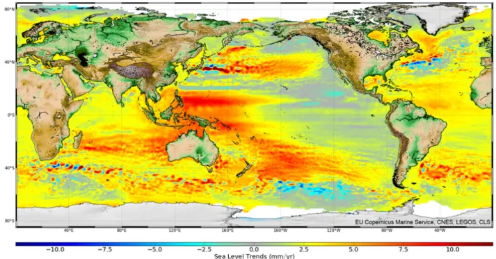
Sea level is not rising uniformly (Fig. 2.1). Satellite altimetry observations, over the last two decades, have revealed that rates of sea level rise at regional scale may differ substantially from the global mean rise. This spatial variability is mostly due to the redistribution of heat, salt and water mass, associated with ocean dynamical processes [Stammer et al., 2013].

Figure 2.1: Spatial trend patterns of altimetry-based global sea level over 1993–2014. Gridded multi-mission SSALTO/DUACS data (from AVISO).

Tide gauges measurements also suggest substantial spatial variations in sea 31

(46)

level. However, tide gauge records are the sum of two components:

• the absolute sea level, the same measured by satellite altimetry, which is the climate-related component of the sea level variability;

• the vertical land motion (VLM) of the tide gauge benchmark, to which the sea level observations are referred.

Any vertical motion at a tide gauge site affects the measured sea level. The VLM can be equal or larger than the local absolute sea level signal, thus masking the climatic-related information of the tide gauge record [Douglas, 2001]. Therefore, the principal difference between the data acquired by satellite altimetry and tide gauges is due to the VLM [Nerem and Mitchum, 2002]. In order to correct the tide gauge records, the vertical land motion need to be estimated; one possible approach is the use of space geodetic techniques [Zerbini et al., 1996; W¨oppelmann et al., 2007]. Among them, the most used is the GPS. While models account only for the GIA, permanent GPS stations, co-located at tide gauge sites, measure accurately and continuously vertical motions.

Figure 2.2 illustrates a tide gauge station co-located with a GPS antenna/receiver and satellite altimetry sea level measurements. The tide gauge measures the rel-ative sea level (S). This record is referred to a ground benchmark which can be subjected to VLM (U); these are estimated by means of GPS data. The satellite altimeter measures the absolute sea level (N), referred to the Earth’s center of mass. The absolute sea level at the tide gauge site can be estimated by

N = S + U (2.1) In the ideal case study presented in the figure, it is assumed that the tide gauge and the satellite are observing the same sea level at the coast and offshore, respec-tively, and that the GPS is measuring the VLM affecting the tide gauge station [W¨oppelmann et al., 2009].

Despite the many efforts done to combine the information from tide gauges and GPS measurements, the availability of co-located GPS stations is still limited [Santamar`ıa-G`omez et al., 2012]. Because of this, the correction of relative sea level trends, using GPS-derived estimates of VLM, requires careful consideration. High-accuracy GPS observations are only available since early-mid 1990s (the ear-liest GPS data in this study begin in 1996). Therefore, to correct tide gauge data collected prior to early 1990s, one should extrapolate to the past a constant GPS-derived VLM rate. It is obvious that this assumption might not be correct,

(47)

2.1. REGIONAL SEA LEVEL AND VERTICAL LAND MOTION 33

Figure 2.2: Scheme of a GPS-equipped tide gauge station and satellite altimetry measurements [From W¨oppelmann et al., 2009].