Involvement of genes and non-coding RNAs in cancer: profiling using microarrays

(1)

Università degli Studi di Ferrara

DOTTORATO DI RICERCA IN

FARMACOLOGIA ED ONCOLOGIA MOLECOLARE

CICLO XXI

COORDINATORE Prof. Pier Andrea Borea

Involvement of genes and non-coding RNAs in

cancer: profiling using microarrays

Settore Scientifico Disciplinare BIO/14

Dottorando Tutore

Dott. ssa Rossi Simona Prof. Volinia Stefano

____________________ ____________________

(firma) (firma)

(2)

(3)

ABSTRACT

MicroRNAs (miRNAs) are small noncoding RNAs (ncRNAs, RNAs that do not code for proteins) that regulate the expression of target genes. MiRNAs can act as tumor suppressor genes or oncogenes in human cancers. Moreover, a large fraction of genomic ultraconserved regions (UCRs) encode a particular set of ncRNAs whose expression is altered in human cancers. Bioinformatics studies are emerging as important tools to identify associations between miRNAs/ncRNAs and CAGRs (Cancer Associated Genomic Regions). ncRNA profiling, the use of highly parallel devices like microarrays for expression, public resources like mapping, expression, functional databases, and prediction algorithms have allowed the identification of specific signatures associated with diagnosis, prognosis and response to treatment of human tumors.

(8)

SUMMARY

The massive production of biological data by means of highly parallel devices like microarrays for gene expression has paved the way to new possible approaches in molecular genetics. Among them the possibility of inferring biological answers by querying large sets of expression data. Based on this principle was implemented TOM, a web-based resource for the efficient extraction of candidate genes for hereditary diseases. The algorithm uses the information stored in public resources, including mapping, expression and functional databases to select one or more candidate genes. This approach allows the geneticist to bypass the costly and time consuming tracing of genetic markers through entire families and might improve the chance of identifying disease genes, particularly for rare diseases. Results were obtained on known benchmark and on hereditary predisposition to familial thyroid cancer.

After TOM project, the efforts were focused on miRNAs study. MiRNAs are small, ncRNAs that can contribute to cancer development and progression by acting as oncogenes or tumor suppressor genes. MiRNAs and UCRs are frequently located at fragile sites and genomic regions affected in various cancers, named cancer associated genomic regions (CAGRs). Bionformatics studies are important tools to identify associations and correlations between miRNAs/ncRNAs and CAGRs. An algorithm was implemented to calculate statistically significant Spearman correlations between UCRs and miRNAs and it supported biological experiments proving that certain UCRs whose expression may be regulated by miRNAs abnormally expressed in human chronic lymphocytic leukaemia (CLL).

Moreover, miRNAs microarray profiling was performed to study and support the hypothesis of a possible miRNA hypermethylaton profile characteristic of human metastasis. A pharmacological and genomic approach was used to reveal aberrant epigenetic silencing program by treating lymph node metastatic cancer cells with a DNA demethylating agent followed by hybridization to an expression microarray. Among the miRNAs that were reactivated upon drug treatment, miR-148a, miR-34b/c, and miR-9 were found to undergo specific hypermethylation –associated silencing in cancer cells compared with normal tissues. The findings indicate that DNA methylation-associated silencing of tumor suppressor miRNAs contributes to the development of human cancer metastasis. The miRNAs microarray profiling contributed to support those results.

(9)

LIST OF PUBLICATIONS

This thesis is based on the following original articles and reviews plus a regional project presented at BITS 2007.

I. GebbaLab project, 2006-2008, www.gebbalab.it

II. Rossi S*, Masotti D, Nardini C, Bonora E, Romeo G, Macii E, Benini L, Volinia S.

(2006) TOM: a web-based integrated approach for identification of candidate

disease genes. Nucleic Acids Res.:W285-92.

III. Masotti D*, Nardini C, Rossi S, Bonora E, Romeo G, Volinia S, Benini L. (2007)

TOM: enhancement and extension of a tool suite for in silico approaches to multigenic hereditary disorders. Bioinformatics. 24(3):428-9.

IV. Gamberoni G, Lamma E, Lodo G, Marchesini J, Mascellani N, Rossi S, Storari S, Tagliavini L, Volinia S*. (2007) Fun&Co: identification of key functional differences

in transcriptomes. Bioinformatics. 23(20):2725-32.

V. Mascellani N*, Liu X, Rossi S, Marchesini J, Valentini D, Arcelli D, Taccioli C, Helmer Citterich M, Liu CG, Evangelisti R, Russo G, Santos JM, Croce CM, Volinia S*. (2007) Compatible solutes from hyperthermophiles improve the quality

of DNA microarrays. BMC Biotechnol. 23;7:82.

VI. Calin GA*, Liu CG, Ferracin M, Hyslop T, Spizzo R, Sevignani C, Fabbri M, Cimmino A, Lee EJ, Wojcik SE, Shimizu M, Tili E, Rossi S, Taccioli C, Pichiorri F, Liu X, Zupo S, Herlea V, Gramantieri L, Lanza G, Alder H, Rassenti L, Volinia S, Schmittgen TD, Kipps TJ, Negrini M, Croce CM. (2007) Ultraconserved regions

encoding ncRNAs are altered in human leukemias and carcinomas. Cancer Cell.

12(3):215-29.

VII. Rossi S, Macellani N, Marchesini J, Gamberoni G, Tagliavini L, Taccioli C, Volinia

S*. (2007) I microRNA: un nuovo attore sul palcoscenico cellulare. Accademia Delle Scienze. Universita’ di Ferrara.

VIII. Rossi S, Sevignani C, Nnadi SC, Siracusa LD, Calin GA*. (2008)

Cancer-associated genomic regions (CAGRs) and noncoding RNAs: bioinformatics and therapeutic implications. Mamm Genome. 19(7-8):526-40. Review

IX. Lujambio A, Calin GA, Villanueva A, Ropero S, Sánchez-Céspedes M, Blanco D, Montuenga LM, Rossi S, Nicoloso MS, Faller WJ, Gallagher WM, Eccles SA, Croce CM, Esteller M*. (2008) A microRNA DNA methylation signature for human

cancer metastasis. Proc Natl Acad Sci U S A. 105(36):13556-61.

X. Rossi S, Calin GA, Amoroso A, Mascellani N, Volinia S*.OMiR: identification of

associations between OMIM diseases and microRNAs. Submitted

XI. Rossi S, Kopetz S, Davuluri R, Hamilton S., Calin GA*. MicroRNAs and

ultraconserved genes: from the scientist bench to the bedside of colorectal cancer patients. Review. Submitted

(10)

INTRODUCTION

Ceaseless advances in biotechnology, along with the growing experience cumulated by researchers in recent years, has allowed a continuous and faster blooming of the number of genomes being sequenced and, most importantly, annotated. The consequent necessities of storing, retrieving, sharing and, in particular, understanding this vast amount of data led to the creation of genome databases, an open source of genetic information for scientists worldwide. Whereas the genomic era opened the doors to the very existence of such large and comprehensive (omic) data repositories, the strongest urgency of the post-genomic era is now to interrelate various sources of biomedical information. Several parallel efforts are currently underway to achieve a better understanding of the human genome. These actions are turned to the extraction of high-throughput information from global approaches such as the International HapMap Project (The International HapMap Consortium, 2005) for identification of single nucleotide polymorphisms or the prosecution of the ENCODE [Encyclopedia Of DNA Elements (ENCODE Consortium, 2004)] for the identification of all functional elements in the genome sequence. Therefore the integration of various existing and upcoming efforts is going to be a key element for the full comprehension of the cellular machinery. We focused on two of the many fields that will strongly benefit from such an integration: the study of hereditary diseases and the study of cancer. Often more than one gene is involved in life threatening misfunctioning of cellular functions. To characterize such diseases the identification of all the responsible genes is eventually a crucial requirement. This process usually involves costly, time consuming and difficult tracing of large family lineages to follow the line of transmission of genes and thus to define the linkage areas where genes responsible for the disease could be located. Computational technologies can appropriately be employed to integrate available data and can, in principle, be used to save on the expensive process of candidate genes selection.

Furthermore, with the advent of high-throughput technologies for the global measurement of miRNAs, these post-transcriptional regulatory molecules are emerging as a new class of cancer biomarkers. Numerous studies have explored associations between miRNAs and cancer features (for a view see Jeffrey 2008).

Discovered in Caenorhabditis elegans in 1993 and formally named in 2001 (Ruvkun 2001), miRNAs have been identified in every plant and animal species examined. They are a class of noncoding RNAs, 18–25 nucleotides in length, that plays key roles in the

(11)

apoptosis and metabolic homeostasis. The functions and targets of most miRNAs await discovery. However, specific miRNAs show expression variation across different stages of organism development, in tissue-specific cell patterning and asymmetry during organogenesis, and in oncogenesis (Garzon et al., 2006). Figure 1 shows the miRNAs biogenesis.

Figure 1. In the nucleus, a primary miRNA (pri-miRNA) is transcribed from DNA by the RNA polymerase II (Pol II) or Pol III enzyme. The long pri-miRNA transcript( 0.5–7kb) folds into a single or a cluster of multiple hairpin structure(s). The pri-miRNA is then cleaved by a microprocessor complex composed of the enzyme Drosha, a nuclear RNase III and the RNA binding protein cofactor Pasha (also known as DGCR8). The shorter stem-loop structure ( 60–70 nucleotides), now termed precursor miRNA (pre-miRNA), is transported across the nuclear membrane by Exportin 5. In the cytoplasm, the pre-miRNA is further processed by a second RNase enzyme, Dicer. The hairpin loop is cropped off the double-stranded RNA, leaving a short miRNA duplex that is unwound by a helicase, cleaved into a mature miRNA ( 18–25 nucleotides), and incorporated into an RNA-induced silencing complex (RISC), with an Argonaute protein as the catalytic component. The miRNA-RISC complex negatively regulates post-transcriptional gene expression by hybridizing to complimentary sequences in the 3' untranslated region (UTR) of a target mRNA and inhibiting protein translation or degrading the mRNA itself. (Figure from Jeffrey SS, Nat Biotechnol. 26:400-401, (2008))

Here I present several algorithms and web applications (TOM, Fun&Co and GebbaLab), implemented by me and my collaborators, to extract knowledge related to hereditary diseases and cancer, from public microarray messengerRNA and annotation data sets, and miRNAs microarray cancer studies. I report also several works which into my statistical analysis and bioinformatics procedures helped to quantify, confirm and visualize hypotheses and results, such as: improve the quality of DNA microarrays, ultraconserved regions encoding ncRNAs are altered in human leukemias and carcinomas, miRNA DNA methylation signature for human cancer metastasis and miRNAs involved in colorectal cancer (CRC).

(12)

DNA microarrays

A DNA microarray is a multiplex technology used in molecular biology and in medicine. It consists of an arrayed series of thousands of microscopic spots of DNA oligonucleotides, called features, each containing picomoles of a specific DNA sequence. This can be a short section of a gene or other DNA element that are used as probes to hybridize a cDNA or cRNA sample (called target) under high-stringency conditions. Probe-target hybridization is usually detected and quantified by fluorescence-based detection of fluorophore-labeled targets to determine relative abundance of nucleic acid sequences in the target.

In standard microarrays, the probes are attached to a solid surface by a covalent bond to a chemical matrix (via epoxy-silane, amino-silane, lysine, polyacrylamide or others). The solid surface can be glass or a silicon chip, in which case they are commonly known as

gene chip. Other microarray platforms, such as Illumina, use microscopic beads, instead

of the large solid support. DNA arrays are different from other types of microarray only in that they either measure DNA or use DNA as part of its detection system.

DNA microarrays can be used to measure changes in expression levels, to detect single nucleotide polymorphisms (SNPs), in genotyping or in resquencing mutant genomes. Microarrays also differ in fabrication, workings, accuracy, efficiency, and cost. Additional factors for microarray experiments are the experimental design and the methods of analyzing the data. Arrays of DNA can be spatially arranged, as in the commonly known gene chip (also called genome chip, DNA chip or gene array), or can be specific DNA sequences labelled such that they can be independently identified in solution. The traditional solid-phase array is a collection of microscopic DNA spots attached to a solid surface, such as glass, plastic or silicon biochip. The affixed DNA segments are known as probes . Thousands of them can be placed in known locations on a single DNA microarray.

DNA microarrays can be used to detect DNA (as in comparative genomic hybridization), or detect RNA (most commonly as cDNA after reverse transcription) that may or may not be translated into proteins. The process of measuring gene expression via cDNA is called expression analysis or expression profiling.

Since an array can contain tens of thousands of probes, a microarray experiment can accomplish that many genetic tests in parallel. Therefore arrays have dramatically accelerated many types of investigation (Table 1).

(13)

Table 1 Microarray Applications Technology or Application Synopsis Gene expression profiling

In an mRNA or gene expression profiling experiment the expression levels of thousands of genes are simultaneously monitored to study the effects of certain treatments, diseases, and developmental stages on gene expression. For example, microarray-based gene expression profiling can be used to identify genes whose expression is changed in response to pathogens or other organisms by comparing gene

expression in infected to that in uninfected cells or tissues. Comparative genomic

hybridization

Assessing genome content in different cells or closely related organisms.

Chromatin

immunoprecipitation on Chip

DNA sequences bound to a particular protein can be isolated by immunoprecipitating that protein (ChIP), these fragments can be then hybridized to a microarray (such as a tiling array) allowing the

determination of protein binding site occupancy throughout the genome. Example protein to immunoprecipitate are histone modifications

(H3K27me3, H3K4me2, H3K9me3, etc), Polycomb-group protein (PRC2:Suz12, PRC1:YY1) and trithorax-group protein (Ash1) to study the epigenetic landscape or RNA Polymerase II to study the transcription lanscape.

SNP detection Identifying single nucleotide polymorphism among alleles within or between populations. Several applications of microarrays make use of SNP detection, including Genotyping, forensic analysis, measuring predisposition to disease, identifying drug-candidates, evaluating germline mutations in individuals or somatic mutations in cancers, assessing loss of heterozygosity, or genetic linkage analysis. Alternative splicing

detection

An exon junction array design uses probes specific to the expected or potential splice sites of predicted exons for a gene. It is of

intermediate density, or coverage, to a typical gene expression array (with 1-3 probes per gene) and a genomic tiling array (with hundreds or thousands of probes per gene). It is used to assay the expression of alternative splice forms of a gene. Exon arrays have a different design, employing probes designed to detect each individual exon for known or predicted genes, and can be used for detecting different splicing isoforms.

Tiling array Genome tiling arrays consist of overlapping probes designed to densely represent a genomic region of interest, sometimes as large as an entire human chromosome. The purpose is to empirically detect expression of transcripts or alternatively splice forms which may not have been previously known or predicted.

(14)

DNA microarray- two colors

DNA microarrays allow for rapid measurement and visualisation of differential expression between genes at the whole genome scale. The major steps involved in this process are:

i. Microarray production process ii. Target preparation

iii. Hybridization iv. Slide scanning

v. Data analysis

vi. Expression profile clustering

Microarray production process

DNA fragments amplified by PCR technique are spotted on a microscopic glass slide coated with polylysine prior to spotting process. The polylysine coating goal is to ensure DNA fixation through electrostatic interactions. Slide preparation is achieved by blocking the polylysine not fixed to DNA in order to avoid target binding. Prior to hybridisation, DNA is denatured to obtained a single strand DNA on the microarray, this will allow the probe to bind to the complementary strand from the target.

Target preparation

RNA are extracted from cultures/samples from which we want to compare expression level. Messengers RNA are then transformed in cDNA by reverse transcription. On this stage, DNA from the first culture with a green dye, whereas DNA from the second culture is labelled with a red dye.

Hybridisation

Green labelled cDNA and red labelled ones are mixed together (call the target) and put on the matrix of spotted single strand DNA (call the probe). The chip is then incubated one night at 60 degrees. At this temperature, a DNA strand that encounter the complementary strand and match together to create a double strand DNA. The fluorescent DNA will then hybridise on the spotted ones (Figure 2).

(15)

Figure 2 Hybridization. (Figure from http://transcriptome.ens.fr/sgdb/presentation/principle.php).

Slide scanning

A laser excites each spot and the fluorescent emission gather through a photo-multiplicator (PMT) coupled to a confocal microscope. We obtained two images where grey scales represent fluorescent intensities read. If we replace grey scales by green scales for the first image and red scales for the second one, we obtained by superimposing the two images one image composed of spots going from green ones (where only DNA from the first condition is fixed) to red (where only DNA from the second condition is fixed) passing through the yellow colour (where DNA from the two conditions are fixed on equal amount).

Data analysis

We have now two microarray images from which we have to calculate the number of DNA molecules in each experimental condition. To do so, we measure the signal amount in the green dye emission wavelength and the signal amount in the red dye emission wavelength. Then we normalise these amount according to various parameters (yeast amount in each culture condition, emission power of each dye, …). We suppose that the amount of fluorescent DNA fixed is proportional to the mRNA amount present in each cell at the beginning and we calculate the red/green fluorescence ratio. If this ratio is greater than 1 (red on the image), the gene expression is greater in the second experimental condition, if this ration is smaller than 1 (green on the image), the gene expression is greater in the first condition as shown in Figure 3.

(16)

Figure 3 Two Color microarray, scatter plot of differentially expressed genes. (Figure from http://transcriptome.ens.fr/sgdb/presentation/principle.php).

Expression profile clustering

Then we can try to gather genes that share the same expression profile on several experiments. This clustering can be done gradually as for phylogenetic analysis, which consist in calculating similarity criteria between expression profiles and gather the most similar ones. We can also use more complex techniques as principal component analysis or neuronal networks.

DNA microarrays – one color - Affymetrix©

The GeneChip high-density oligonucleotide arrays are fabricated by using in-situ synthesis of short oligonucleotide sequences on a small glass chip using light directed synthesis. This technique allows for the precise construction of a highly ordered matrix of DNA oligomers on the chip.

Design overview

In the GeneChip system a known gene or potentially expressed sequence is represented on the chip by 11-20 unique oligomeric probes, each 25 bases in length. The group of probes corresponding to a given gene or small group of highly similar genes is known as the probe set and generally spans a region of about 600 bases, known as the target sequence. Many copies of each oligomer are synthesized in discrete features (or cells) on the GeneChip array. In addition, for each oligomer on the array there is a

(17)

mismatched base at the central position (i.e. base 13). These are designated Perfect Match (PM) and Mismatch (MM) probes, respectively. The MM probes serves as a control for non-specific hybridization.

GeneChip Array Fabrication

Probe arrays are manufactured by Affymetrix's proprietary, light-directed chemical synthesis process, which combines solid-phase chemical synthesis with photolithographic fabrication techniques employed in the semiconductor industry. Using a series of photolithographic masks to define chip exposure sites, followed by specific chemical synthesis steps, the process constructs high-density arrays of oligonucleotides, with each probe in a predefined position in the array. Multiple probe arrays are synthesized simultaneously on a large glass wafer. This parallel process enhances reproducibility and helps achieve economies of scale. The wafers are then diced, and individual probe arrays are packaged in injection-molded plastic cartridges, which protect them from the environment and serve as chambers for hybridization.

Data Overview

Affymetrix GeneChip experiments are managed using GCOS. GCOS interfaces with equipment to run a probe array experiment and is also used to generate preliminary analysis data from an experiment. The next section covers the basics of files generated by GCOS and also explains some of the most widely used variables generated by GCOS.

MAS File Types

The next section covers the basics of files generated by GCOS and also explains some of the most widely used variables generated by GCOS.

• Experiment File *.EXP: This file contains the parameters of the experiment such as Probe Array Type, Experiment Name, Equipment parameters, Sample Description, and others. This file is not used for analysis, but is required to open other GCOS files for the designated chip experiment.

• Image Data File *.DAT: This is an image file generated by the scanner from the Probe Array after processing on the Fluidics Station. This file can be viewed in GCOS to assess the quality of scanning event or exported as a *.TIFF image. It is used in GCOS to generate the *.CEL file.

• Cell Intensity File *.CEL: This binary file is the result of low level analysis performed from the *.DAT image file. It is exported from GCOS and is often used as the base file

(18)

for further analysis.

• Probe Array Results File *.CHP: This binary file is a gene level summarization of the CEL file using the Affymetrix’ MAS 5.0 or PLIER algorithms. It is exported from GCOS. It can also be used as the base file for further analysis; however one needs to know the settings of key parameters (alpha1, alpha2, tau, target signal etc.). There are many other algorithms that have been adopted by the community other than MAS 5.0 and PLIER, hence the reason why CEL files are often preferred over CHP files by Investigators for analysis.

• Report File *.RPT: The report file is generated from the chip file. This expression report summarizes information about expression analysis settings and probe set hybridization intensity data.

• MAGE-ML *.XML: This file contains information related the microarray experiment (one per experiment). This information can include biologically relevant information, array details, fluidics protocol details and the analysis settings. It also records the file hierarchy of an experiment.

GCOS uses a statistical algorithm to calculate signals and make significance calls for the data: MAS (MAS 5.0 computes local background in each of 16 squares, and then subtracts a weighted combination of these background estimates from each probe intensity).

MAS Analysis Metrics

• Signal: a measure of the abundance of transcript

• Detection: the call that indicates whether the transcript is detected (P present),

undetected ( A, absent), or at the limit of detection (M, marginal).

• Detection p-value: p-value that indicates the significance of the detection call. • Signal Log Ratio: the change in expression level of a transcript between a

baseline and an experiment array. This change is expressed as the log2 ratio.

Each probe set on a GeneChip array has a unique name known as the Probe set ID.

Affymetrix has upgraded their MicroArray Suite (MAS) software several times. MAS 4.0 was the standard until January 2002 and is still cited in published papers. MAS 4 calculates a weighted average of the probe-pair differences (PM – MM) for each probe pair representing a gene. MAS 5.0 improves in two important ways. First the intensities are transformed to a logarithmic scale before the average is taken; this equalizes the

(19)

contribution of different probes. Secondly an estimate of background based on MM replaces MM itself in the difference PM-MM; this estimate is itself a weighted average of log probe pair differences: log(PMj/MMj).

Normalization

Biologists have long experience coping with systematic variation between experimental conditions (technical variation) that is unrelated to the biological differences. Normalization is the attempt to compensate for systematic technical differences between chips, to see more clearly the systematic biological differences between samples. For example, differences in treatment of two samples, especially in labelling and in hybridization, bias the relative measures on any two chips.

Normalization by Scaling and its Limitations

The simplest approach to normalizing Affymetrix data is to re-scale each chip in an experiment to equalize the average (or total) signal intensity across all chips. The reasoning behind this is that there should be with equal weights of RNA for all the samples; if the sizes of the RNA molecules are comparable, the number of RNA molecules should also be the roughly the same in each sample. Consequently, nearly the same number of labeled molecules from each sample should hybridise to the arrays and, if all other conditions were equal, the total hybridisation intensities summed over all elements in the arrays should be the same for each sample.

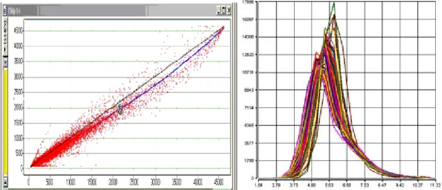
To do better, we examine in detail the relationships among replicate chips (chips hybridized to the same sample). Figure 4a shows a scatter plot of probes from one pair of chips; there is clearly a non-linear relation among probes. Figure 4b shows plots of probe distributions from a number of replicate chips on a log scale; these distributions have very different shapes; on a log scale, applying a scaling transform to a chip, shifts its distribution curve to the right or left, but doesn't change its shape.

(20)

Figure 4. a) Plot of probe signals from two Affymetrix chips hybridized with identical mRNA samples. The black straight line represents equality, while the blue curve is a spline fit through the scatter plot. B) Density curves of global signal intensities. The plots show the overall signal density distribution of all probe sets represented on the HG-U133 Plus 2.0 microarray. Data from each microarray analysis is represented by a separate line. The plot is useful to visualize whether there are differences in the overall signal distributions of the experiments. (Figure from http://www.bea.ki.se/staff/reimers/Web.Pages/Affymetrix.Normalization.htm).

Quantile Normalization

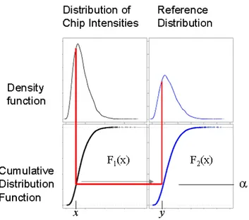
Is a non-parametric procedure normalizing to a synthetic chip (Bolstad et al., 2003). It is a kind of normalization that works across arrays as well as within arrays. It turns out that quantile normalization works quite well at reducing variance between arrays, while compensating the intensity-dependent dye bias, as well as does lowess normalization.This method assumes that the distribution of gene abundances is nearly the same in all samples. The pooled distribution of probes on all chips are taken. Then to normalize each chip the algorithm compute for each value, the quantile of that value in the distribution of probe intensities; then it transform the original value to that quantile's value on the reference chip. In a formula, the transform is

xnorm = Fi-1(Fref(x)) ,

where Fi is the distribution function of chip i, and Fref is the distribution function of the

(21)

Figure 5. Schematic representation of quantile normalization: the value x, which is the α-th quantile of all probes on chip 1, is mapped to the value y, which is the α quantile of the reference distribution F2. (Figure from http://www.bea.ki.se/staff/reimers/Web.Pages/Affymetrix.Normalization.htm).

Proportional Variance – RMA (Robust Multichip Average)

This is largely the work of Terry Speed's group at Berkeley, especially Ben Bolstad, and Rafael Irizarry (Irizarry et al., 2003). They work only with PM values, and ignore MM entirely. They take a log transform of equation () and find:

With errors proportional to intensity in the original scale, the errors on the log scale have constant variance. After background subtraction and normalization they fit:

where nlog is their terminology for 'normalize and then take logarithm'. They fit this model by iteratively re-weighted least squares, or by median polish. Code is available in the affy package on BioConductor, together with quantile normalization (http://www.bioconductor.org/packages/bioc/).

(22)

Figure 6. Raw Data Box Plot (left), the same intensity box plot using normalized data (right). The normalization remove effects seen in large proportions of the data (in this case a time effect is obvious) while still preserving effects seen in small proportions of the data. (Figure from http://bioinf.wehi.edu.au/affylmGUI/R/library/affylmGUI/doc/estrogen/estrogen.html).

GCRMA

Another proposed background correction method is GC-RMA (Wu et al., 2003). This method is based upon sequence information, such as GC content, for each probe and stochastic models for binding affinities. GC-RMA is a modified version of RMA that models intensity of probe level data as a function of GC-content. We expect to see higher intensity values for probes that are GC rich due to increased binding.

Exploratory Analysis

Pattern-Finding

Exploratory analysis aims to find patterns in the data that aren’t predicted by the experimenter’s current knowledge or pre-conceptions. Some typical goals are to identify groups of genes expression patterns across samples are closely related; or to find unknown subgroups among samples. A useful first step in all analyses is to identify outliers among samples – those that appear suspiciously far from others in their group. To address these questions, researchers have turned to methods such as cluster analysis, and principal components analysis.

Clustering

(23)

profiles are like distances; however the user must make choices to compute a single measure of distance from many individual differences. Different procedures emphasize different types of similarities, and give different resulting clusters. Four choices we have to make are:

i. what scale to use: original scale, log scale, or another transform, ii. whether to use all genes or to make a selection of genes,

iii. what metric (distance measure) to use to combine the scaled values of the selected genes,

iv. what clustering algorithm to use.

Scale

Differences measured on the linear scale will be strongly influenced by the one hundred or so highly expressed genes, and only moderately affected by the hundreds of moderate abundance genes; the thousands of low abundance genes will contribute little. Often the high-abundance genes are 'housekeeping' genes; these may or may not be diagnostic for the kinds of differences being sought. On the other hand, the log scale will amplify the noise among genes with low expression levels. If low-abundance genes are included then they should be down-weighted. The most useful measure of a single gene difference is the difference between two samples, relative to that gene's variability within experimental groups: this is like a t-score for difference between two individuals.

Gene Selection

It would be wise not to place much emphasis on genes whose values are uncertain. These are usually those with low signals in relation to noise, or which fail spot-level quality control. If the estimation software provides a measure of confidence in each gene estimate, this can be used to weight the contribution to distance of that gene overall. It's not wise to simply omit (that is, set to 0) distances which are not known accurately, but it is wise to down-weight relative distances if several are probably in error. A simple general rule is that genes whose signal falls within the background noise range are probably contributing just noise to your clustering (and any other global procedure); discard them.

Metrics

Usually, cluster programs give us a menu of distance measures: Euclidean, Manhattan distances, and some relational measures: correlation, and sometimes relative distance, and mutual information. The names describe how differences are combined:

(24)

Euclidean is straight-line distance: (root of sum of squares, as in geometry), Manhattan is sum of linear distances (like navigating in Manhattan). The correlation distance measure is actually 1-r, where r is the correlation coefficient. Probably a more useful version is 1 – |r|; negative correlation is as informative as positive correlation. We do get different results depending on the algorithm we use, as shown below (Figure 7) for a study with 10 samples: two normal samples and two groups of tumor samples.

Figure 7 Clustering of the same data set using four different distance measures. (Figure from http://discover.nci.nih.gov/microarrayAnalysis/Exploratory.Analysis.jsp).

Principal Components and Multi-dimensional scaling

Several other good multivariate techniques can help with exploratory analysis. Many authors suggest principal components analysis (PCA) or singular value decomposition to find coherent patterns of genes, or ‘metagenes’, that discriminate groups. These techniques with a long history in the statistical arsenal rely on the idea that most variation in a data set can be explained by a smaller number of transformed variables; they each form linear combinations of the data, which represent most of the variation, and in principle these approaches, are well-suited for this purpose. These multivariate approaches are more useful for exploring relations among samples, and particularly for a

(25)

diagnostic look at samples before formal statistical tests (see Figure 8).

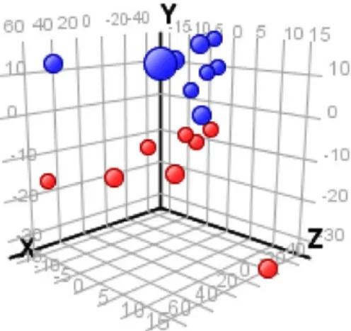
Figure 8 shows a GeneSpring© PCA plot of two groups in a comparative study; the control group is in red; treated samples are quite distinct from untreated and each other. (Figure obtained using 16 samples of treated and untreated samples).

Statistical Tests

The Purposes of Statistical Tests

Microarray studies often aim to identify genes that are differentially regulated across different classes of samples; examples are: finding the genes affected by a treatment, or finding marker genes that discriminate diseased from healthy subjects.

Microarray data is often used as a guide to further, more precise studies of gene expression by qt-PCR or other methods. Then the goal of the statistical analysis is heuristic: to provide the experimenter with an ordered list of good candidate genes to follow up. Sometimes the experimenter plans to publish microarray results as evidence for changes in gene abundance; in this case it is important to state the correct degree of evidence: the ‘p-value’. Being many genes actually tested in parallel singles p-values are wrong in the context of testing thousands of genes. A better way to specify the confidence of microarray results is the ‘false discovery rate’.

Transforms

Often the first step is transforming the values to log scale, and doing all subsequent steps on the log-transformed values. Although taking logarithms is common practice, and

(26)

helpful in several ways, there are other options. The main justification for transforms in statistics is to better detect differences between groups whose within-group variances are very different. Most commonly the within-group variances are higher in those groups where the mean is also higher. A different kind of variation, the measurement error in expression level estimates, grows with the mean level. If the measurement error is proportional to the mean, then the log-transformed values will have consistent variance for all genes. For both reasons many researchers argue that gene expression measures should be analyzed on a logarithmic scale.

Comparison of Two Groups of Samples

The simplest and most common experimental set-up is to compare two groups: for example, Treatment vs. Control, or Mutant vs. Wild type.

The long-time standard test statistic for comparing two groups is the t-statistic:

t = (xi,1 – xi,2) / si,

where xi,1 is the mean value of gene i in group 1, xi,2 is the mean in group 2, and si is

the (non-pooled) within-groups standard error (SE) for gene i.

Another approach to detecting more of the differentially expressed genes is to use a more precise estimate of the variation between individuals, for each gene, in tests of that gene. If a good deal of prior data exist on the tissue and strain used in the wild-type (or control) group, measured on the same microarray platform – and this is sometimes the case now – then it is defensible to pool the estimates of wild-type variation from each of the prior studies, and use this as the denominator in the t-scores. The t-scores should then be compared to the t-distribution on a number of degrees of freedom, equal to that used in computing the pooled standard error. A variant of this approach may be used in a study where many groups are compared in parallel. The within-group variances for each gene may be pooled across the different groups to obtain a more accurate estimate of variation. This presumes that treatments applied to different groups affect mostly the mean expression levels, and not the variation among individuals. Of course one should test that the discrepancies in variance estimates are not too large for many of the genes that are selected as differentially expressed. This may be done by computing the ratios of variances between groups (F-ratios), and comparing to an F-distribution.

(27)

Permutation Tests

Permutation testing is an approach that is widely applicable and copes with distributions that are far from Normal; this approach is particularly useful for microarray studies because it can be easily adapted to estimate significance levels for many genes in parallel. Some recent software packages, notably SAM (Significance Analysis of Microarray, http://www-stat.stanford.edu/~tibs/SAM/), implement permutation testing in a menu-driven interface.

The meaning of a p-value from a permutation procedure differs from the meaning of a model-based p-value. The model-based p-value is the probability of the test statistic, assuming that the gene levels in both the treatment and control groups follow the model (eg. a Normal distribution). A permutation-based p-value tells how rare that test statistic is, among all the random partitions of the actual samples into pseudo-treatment and pseudo-control groups. The steps in a permutation-based computation of the significance level of a test statistic are as follows:

i. Choose a test statistic, eg. a t-score for a comparison of two groups, ii. Compute the test statistic for the gene of interest,

iii. Permute the labels on samples at random, and re-compute the test statistic for the rearranged labels; repeat for a large number (perhaps 1,000) permutations, and finally,

iv. Compute the fraction of cases in which the test statistics from iii) exceed the real test statistic from ii).

Volcano Plot

However one chooses to compute the significance values (p-values) of the genes, it is interesting to compare the size of the fold change to the statistical significance level. The ‘volcano plot’ arrange genes along dimensions of biological and statistical significance. The first (horizontal) dimension is the fold change between the two groups (on a log scale, so that up and down regulation appear symmetric), and the second (vertical) axis represents the p-value for a t-test of differences between samples (most conveniently on a negative log scale – so smaller p-values appear higher up). The first axis indicates biological impact of the change; the second indicates the statistical evidence, or reliability of the change. In this way we can then make judgements about the most promising

(28)

candidates for follow-up studies, by trading off both these criteria by eye (Figure 9).

Figure 9. A volcano plot. Siaplaying entities satisfying p_value cutoff and Fold Change cut-off. (Figure obtained using 16 samples of treated and untreated samples).

Genome-Wide Comparisons, Corrected P-Values, and False Discovery Rates

P-Values and False Discovery Rates

Most scientific papers quote p-values, however few papers discuss their meaning. In order to understand what the problem is with quoting p-values for massively parallel comparisons, we need to be precise. Let’s consider, for example, a t-test of differences between two samples. If there is no systematic (real, reproducible) difference between groups, nevertheless the t-score for differences between groups is never exactly 0. Common sense cannot decide whether a particular value provides strong evidence for a real difference. The natural question to ask is: how often a random sampling of a single group would produce a t value as far from 0 as the t we observed. When you declare an effect is significant at 5%, you say you are willing to let one false positive sneak in, roughly every twenty tests. We don’t accept this for critical decisions; we won’t long continue to cross the street, if we do so on a 95% confidence that there is a break in traffic. We may call this the false positive rate (FPR); the FPR of a procedure is the fraction of truly unchanged genes which appear as (false) positives.

If the aim of the microarray study is to select a few genes for more precise study, then the goal is an ordered list of genes, most of which are really different (true positives).

(29)

fraction (for example less than .3) of the genes selected. This goal leads naturally to specifying the false discovery rate (FDR) for a list, rather than significance level (FPR). The FDR is the expected fraction of false positives in a list of genes selected following a particular statistical procedure.

Multiple Testing P-Values and False Positives

Suppose you compare two groups of samples drawn from the same larger group, using a chip with 10,000 genes on it. On average 500 genes will appear ‘significantly different’ at a 5% threshold. For these genes, the variation between samples will be large relative to the variation within groups due to random, but uneven allocation of the expression values to the treatment and control groups. Therefore the p-value appropriate to a single test situation is inappropriate to presenting evidence for a set of changed genes.

Statisticians have devised several procedures for adjusting p-values to correct for the multiple comparisons problem. The oldest is the Bonferroni correction; this is available as an option in many microarray software packages. The corrected p-value, pi* for gene i is

set to: pi* = Npi, if Npi < 1, or 1, if Npi > 1; where pi is the p-value for a single test of gene

i, and N is the number of genes being tested (which may be less than the number of genes on the array).

Calculating Permutation-Based Corrected P-values

To calculate corrected p-values, first calculate single-step p-values for all genes: p1,

…, pN. Then order the p-values: p(1), …, p(N), from least to greatest. Next permute the

sample labels at random, and compute the test statistics for all genes between the two (randomized) groups. For each position k, keep track of how often you get at least one p-value more significant than p(k), from gene k, or from any of the genes further down on the

list: k+1, k+2, …, N. After all permutations, compute the fraction of permutations with at least one apparently more significant p-value less than p(k). This is the corrected p-value

for gene k. Although this procedure is complicated, it is much more powerful than the other corrections: that is, the procedure gives a much smaller corrected p-value for each gene than the Bonferroni procedure, and therefore a bigger list of significant genes at any corrected significance level (specified risk of false positives). This is known as the Westfall–Young correction.

(30)

Several Groups – Analysis of Variance

Many current microarray studies compare more than two groups. Sometimes the question is to determine differences among three or more cell lines, or strains of experimental animal. Another common design compares the effect of a particular treatment (often a ligand for a receptor), on cell lines (or animals) with wild-type and mutant versions of the receptor. Usually the experimenter wants to know which genes are actively regulated during treatment in both cell lines, or wants some criterion for selecting those that are differentially regulated among groups. These questions belong in the tradition of analysis of variance (ANOVA). Generally, all of the procedures that were discussed above in the context of two-sample comparisons, carry over to analogues in ANOVA.

(31)

Microarray databases

There are many public databases for microarray data. The databases meant to be central repositories, among them, the most known:

i. ArrayExpress at EBI (http://www.ebi.ac.uk/arrayexpress/)

ii. GEO (Gene Expression Omnibus) at NCBI (http://www.ncbi.nlm.nih.gov/geo/) They are not only public archives of microarray data but also enforcing standards to maintain data quality, providing powerful search methods to facilitate finding particular data, and providing analytical tools to facilitate comparison and/or visualization of large data. According to the publication about GEO (Barrett et al., 2005), “These data include single and multiple channel microarray-based experiments measuring the abundance of mRNA, genomic DNA and protein molecules. Data generated by innovative applications of microarray technology are also accepted, e.g. chromatin immunoprecipitation (ChIP-chips) for identifying protein-binding DNA regions and tiling arrays for genome annotation. Data from non-array-based highthroughput functional genomics and proteomics technologies are also archived, including serial analysis of gene expression (SAGE), and mass spectrometry peptide profiling.” So, it is not only microarray data.

Let’s look at GEO(Figure 10).

Figure 10 ncbi/GEO query interface. (Figure obtaine from http://www.ncbi.nlm.nih.gov/geo/).

We see we can make queries to get data of our interest or browse through them. The data sets are called GEO-DataSets. It is an experiment-centric view (organized according

(32)

to each experiment). If, for example, we search for “Human[Organism] AND microRNAs” we obtain several records. Note that there are ‘GDS…’ records lines, ‘GSE…’ records, and a ‘GPL…’ record. Each GDS (dataset) record is the entire set of data from one experiment and comes with various tools to play. GSE (series) records explain the experiment, including RNA samples used. GPL (platform) records are descriptions of microarray platforms. We can also see ‘GSM…’ in GDS and GSE records. GSM (sample) records contain data from each sample used in the experiment.

List of several useful microarray data and not only:

• ArrayExpress—a public database of microarray experiments and gene expression profiles

• The Stanford Microarray Database

• Microarray retriever: a web-based tool for searching and large scale retrieval of public microarray data

• OligoArrayDb: pangenomic oligonucleotide microarray probe sets database

• CEBS—Chemical Effects in Biological Systems: a public data repository integrating study design and toxicity data with microarray and proteomics data • Gene Aging Nexus: a web database and data mining platform for microarray data

on aging

• ChipInfo: software for extracting gene annotation and gene ontology information for microarray analysis

• ITTACA: a new database for integrated tumor transcriptome array and clinical data analysis

• BarleyBase—an expression profiling database for plant genomics

• ArrayXPath: mapping and visualizing microarray gene-expression data with integrated biological pathway resources using Scalable Vector Graphics

• NASCArrays: a repository for microarray data generated by NASC’s transcriptomics service

• CanGEM: mining gene copy number changes in cancer

• CleanEx: a database of heterogeneous gene expression data based on a consistent gene nomenclature

• GEPAS: a web-based resource for microarray gene expression data analysis • NetAffx: Affymetrix probesets and annotations

The term microarray database is usually used to describe a repository containing microarray gene expression data. The key features of a microarray database are to store

(33)

the measurement data, manage a searchable index, and make the data available to other applications for analysis and interpretation (either directly, or via user downloads).

Microarray databases can fall into two distinct classes:

i. A peer reviewed, public repository that adheres to academic or industry standards and is designed to be used by many analysis applications and groups. A good example of this is the Gene Expression Omnibus (GEO) from NCBI or ArrayExpress from EBI.

ii. A specialized repository associated primarily with the brand of a particular entity (lab, company, university, consortium, group), an application suite, a topic, or an analysis method, whether it is commercial, non-profit, or academic. These databases may be characterized by:

• A subscription or license may be needed to gain full access,

• The content may come primarily from a specific group (e.g. SMD, or UPSC-BASE),

• There may be limits on how who can use the data, and for what purpose,

• Special permission may be required to submit new data, or there may be no obvious process at all,

• Only certain applications may be equipped to use the data, often also associated with the same entity (for example, caArray at NCI is specialized for the caBIG),

• Further processing or reformatting of the data may be required for standard applications or analysis,

• They claim to address the 'urgent need' to have a standard, centralized repository for microarray data. (See YMD, last updated in 2003, for example),

• There is a claim to an incremental improvement over one of the public repositories,

• A meta-analysis application, which incorporates studies from one or more public databases (e.g. Gemma primarily uses GEO studies; NextBio uses various sources)

Some of the most known public, curated microarray databases are reported in Table

(34)

Table 2 Microarray Databases

Database Scope Web site

Gene Expression Omnibus - NCBI

any curated MIAME compliant molecular abundance study

http://www.ncbi.nlm.nih.gov/geo/

Stanford Microarray database

stores raw and normalized data from microarray experiments, and provides data retrieval, analysis and visualization

http://genome-www5.stanford.edu/

Genevestigator database

Manually curated microarray data for expression meta-analysis

https://www.genevestigator.ethz.ch/gv/index.js p

ArrayExpress at EBI Any curated MIAME or MINSEQE compliant transcriptomics data

http://www.ebi.ac.uk/microarray-as/ae/

UPenn RAD database

MIAMI compliant public and private studies, associated with ArrayExpress

http://www.cbil.upenn.edu/RAD/php/index.php

UNC Microarray database

microarray data storage, retrieval, analysis, and visualization

https://genome.unc.edu/

MUSC database repository for DNA microarray data generated by MUSC investigators

http://proteogenomics.musc.edu/ma/musc_ma db.php?page=home&act=manage

caArray at NCI Cancer data, prepared for analysis on caBIG

https://array.nci.nih.gov/caarray/home.action

UPSC-BASE data generated by microarray analysis within Umeå Plant Science Centre (UPSC).

(35)

MicroRNAs

MicroRNAs (miRNAs) are small noncoding RNAs (ncRNAs, RNAs that do not code for proteins) that regulate the expression of target genes at the posttranscriptional or posttranslational level. Many miRNAs have conserved sequences between distantly related organisms, suggesting that these molecules participate in essential developmental and physiologic processes. miRNAs can act as tumor suppressor genes or oncogenes in human cancers. Mutations, deletions, or amplifications have been found in human cancers and shown to alter expression levels of mature and/or precursor miRNA transcripts. Moreover, a large fraction of genomic ultraconserved regions (UCRs) encode a particular set of ncRNAs whose expression is altered in human cancers.

In genetics, miRNAs are single-stranded RNA molecules of about 21–23 nucleotides in length, which regulate gene expression. miRNAs are encoded by genes from whose DNA they are transcribed but miRNAs are not translated into protein (non-coding RNA); instead each primary transcript (a pri-miRNA) is processed into a short stem-loop structure called a pre-miRNA and finally into a functional miRNA.

Mature miRNA molecules are partially complementary to one or more messenger RNA (mRNA) molecules, and their main function is to down-regulate gene expression. They were first described in 1993 by Lee and colleagues in the Victor Ambros lab (Lee et al., 1993), yet the term microRNA was only introduced in 2001 in a set of three articles in Science (Ruvkun , 2001).

Microarrays for miRNA

The microRNAs expression study had in the past years large difficulties due to their small dimensions and the insufficient sensibility of the methods used, like the Northern blot, the cloning and the arrays on membrane revealed with a radioactive. The application of the technology of the microarrays to the analysis of the profile of expression of miRNA offered meaningful advantages like a greater sensibility and elevated comparative abilities. In the laboratory of Prof. Croce (OSUCCC, Ohio State University, Liu et al., 2008) has been developd a microarray (or chip) for the study of the alterations in the expression of all the miRNA known in the human cancer and it has been established as a reproductable detection method (Liu et Al, 2004). The levels of miRNA are obtained for quantification of the intensities of mark them with appropriate software as GenePix (Figure 11).

(36)

Figure 11. Phases of miRNA microarray experiment. (Figure from paper VII).

MiRNA and cancer

Several miRNAs has been found to have links with some types of cancer.

Recent studies demonstrated that in cancer the levels of some miRNA are altered (Volinia et al., 2006; Lu et al., 2005). Some miRNA, as miR-21 and miR-155 are overexpressed in solid tumors and in the leukaemias. In figure 12 6 solid tumors are represented (columns), and in every line the microRNA associated to the solid tumors. The figure is a graphical rapresentation of the obtained result by using approximately 500 biopsies. A red square represents an overexpression of the microRNAs in tumor; a green represents downregulation of the miRNA in tumor. For example, miR-21 is overwxpressed in all and the 6 considered tumors (breast, lung, colon, pancreas, prostate and stomach).

Figura 12. Fold changes (cancer vs. normal) of the miRNAs present in the signatures of at least 50% of the solid tumors. The tree displays the log2 transformation of the average fold changes (cancer over normal). The mean was computed over all samples from the same tissue or tumor histotype. Arrays were mean centered and normalized by using GENE CLUSTER 2.0. Average linkage clustering was performed by using uncentered correlation metric. (Figure from Volinia S et al., Proc Natl Acad Sci U S A., 103:2257-2261, (2006)).

(37)

The discovery of the association miRNA-cancer although revealed of a strong correlation, has not been enougth to establish a cause-effect connection. After, the responsibility of the microRNA in the insorgence of the cancer has been demonstrated in transgenic mouse with miR-155 (Costinean et al., 2006). In such mice in fact the insertion of additional copies of miR-155 provokes a high grade lymphoma with correspondent splenomegaly (Figure 13).

Figura 13. Transgenic mice, 6 months old, presented an enlarged abdomen and important splenomegaly. (A) Transgenic mice, 6 months old, had a considerably enlarged abdomen compared with wild-type mice, due to the clinically evident splenomegaly. (B) Spleens of the mice shown in A. The transgenic spleen is enlarged due to expansion of leukemic_lymphoma cells. (Figure from Costinean et al., Proc Natl Acad Sci U S A. 103:7024-7029, (2006)).

Moreover, for many genetic diseases, even if studied for a long time and for which the chromosomic region of linkage is well known, the gene- disease has not yet has discovered. For this group of genetic diseases has been hypotized a role of not conventional genes" , like miRNAs.

MiRNAs as cancer players – a balance between miRNA targets repression and miRNA expression regulation.

The classical models of tumorigenesis postulate alterations in protein coding oncogenes and tumor suppressor genes. MiRNAs are also contributors to oncogenesis, functioning as tumor suppressors, as is the case of miR-15a and miR-16-1 (Cimmino et al., 2005) or let-7 family (Johnson et al., 2007)) or as oncogenes, as is the case of

miR-155 (Volinia et al., 2006), miR17-92 cluster (He L et al., 2005) or miR-21 (Chan et al.,

(38)

Relatively minor variations in the levels of expression of a miRNAs or mutations that affect moderately the conformation of miRNA::mRNA pairing could have important consequences for the cell because of the large number of targets of each miRNA. “Traditional teaching” suggests that miRNA binds to target messenger RNA by imperfect complementarity, causing either mRNA degradation, or translation inhibition (Mathonnet et al. 2007). Recently, a deviation from the above point of view on miRNA function was found: the miR-369-3 can up-regulate translation tumor necrosis factor alpha (TNFa) after binding the 3’ untranslated region of TNFa, suggesting an additional level of complexity on miRNA function (Vasudevan et al., 2007).

A growing list of publications proved that miRNAs play a critical role in cancer initiation and progression, and that miRNA alterations are ubiquitous in human cancers. Consequently, events activating or inactivating miRNAs were viewed to cooperate with protein coding genes (PCGs) abnormalities in human tumorigenesis (Calin and Croce, 2006). For example, recently it was shown by Nagel and colleagues that miR-135a and

miR-135b directly target the 3' untranslated region of APC, suppress its expression, and

induce downstream Wnt pathway activity (Nagel et al, 2008). Inactivation of the adenomatous polyposis coli (APC) gene is a major initiating event in colorectal tumorigenesis. Thus, these results uncover a miRNA-mediated mechanism for the control of APC expression and Wnt pathway activity, and suggest its contribution to colorectal cancer pathogenesis.

Much less was known about the upstream regulation of miRNA in cancer cells until recently, when a series of publications demonstrated that the TP53 tumor suppressor regulates the transcription of the miR-34 family (for a review see He X et al., 2007), and that the miR-34 family subsequently mediates induction of apoptosis, cell cycle arrest, and senescence. Using quantitative RT-PCR analysis, it was demonstrated that miR-34a was highly up-regulated in a human colon cancer cell line, HCT 116, treated with a DNA-damaging agent, adriamycin (Tazawa et al., 2007). Furthermore, it was shown that widespread miRNA repression by Myc contributes to tumorigenesis in general (Chang et al., 2008), and to repression of the miR17-92 cluster in particular. MiRNAs from this cluster modulate tumor formation and function as oncogenes by influencing the translation of E2F1 mRNA (O’Donnell et al., 2005).

MicroRNAs and Colorectal Cancer

Cancer is a complex genetic disease caused by the accumulation of mutations, which lead to deregulation of gene expression and uncontrolled cell proliferation. Given

(39)

miRNAs have been implicated in cancer (Bueno et al., 2008). CRC accounts for 13% of all cancers and is the second most common cause of cancer death in the Western world (Aaltonen and Hamilton, 2000, Greenlee and et. 2001, Parkin et al, 2005). Early detection provides a significant survival advantage, and many efforts are focused on improving detection rates and screening utilization. Currently, surgery is the only curative approach for early stage adenocarcinomas, with chemotherapy providing a modest incremental survival benefit at the cost of additional toxicities (Rodriguez-Bigas et al., 2006)(Kopetz et al,, 2008). Therefore, the identification of improved diagnostic and prognostic markers as well as new therapeutic options for CRC patients is of great and immediate interest.

(40)

Cancer-associated genomic regions (CAGRs) and noncoding

RNAs

MiRNAs and UCRs are frequently located at fragile sites and genomic regions affected in various cancers, named cancer-associated genomic regions (CAGRs). Bioinformatics studies are emerging as important tools to identify associations and/or correlations between miRNAs/ncRNAs and CAGRs. ncRNA profiling has allowed the identification of specific signatures associated with diagnosis, prognosis, and response to treatment of human tumors. Several abnormalities could contribute to the alteration of miRNA expression profiles in each kind of tumor and in each kind of tissue. Here we focused on the miRNAs and ncRNAs as genes affecting cancer risk, and we provided an updated catalog of miRNAs and UCRs located at fragile sites or at cancer susceptibility loci. These types of studies are the first step toward discoveries leading to novel approaches for cancer therapies.

Noncoding RNAs and bioinformatics

Recent biotechnology advances, along with a growing number of new biological-computational approaches, have allowed an expansion of the number of genomes being sequenced and annotated, as well as facilitated the development of databases to collect and analyze large amounts of genetic information. The consequent necessities of retrieving, sharing, and, in particular, understanding this vast amount of data led to the creation of genome databases, providing an open source of genetic information for scientists worldwide. Thus, there is now a strong urgency to integrate various sources of biomedical and clinical information.

One of the many fields that will strongly benefit from such integration is the study of noncoding RNAs (ncRNAs) (Barbarotto et al. 2008; Calin and Croce 2006; Esquela-Kerscher and Slack 2006). The most studied ncRNAs are the miRNAs. Recently, the physiologic role of miRNAs during development, differentiation, cell cycle regulation, aging, and metabolism has begun to be elucidated (Ambros 2004; Costa 2005; Johnson et al. 2007; Mendell 2005). Consequently, miRNA deregulation has been found in many different human diseases, including cancer, diabetes, and immuno- or neurodegenerative disorders (Perwez Hussain and Harris 2007; Sevignani et al. 2006). Several lines of evidence implicate abnormalities in miRNA and ncRNA gene expression with cancer, such as (1) the location of ncRNAs at CAGRs, (2) the epigenetic regulation of miRNA expression, and (3) abnormalities in miRNA processing genes and proteins. A unique and specific miRNA signature is able to distinguish between different normal tissues, and