View of Time series outlier detection: a new non parametric methodology (washer)

TIME SERIES OUTLIER DETECTION:

A NEW NON PARAMETRIC METHODOLOGY (WASHER) Andrea Venturini

1. INTRODUCTION

A definition of outlier may be that of Bartnett and Lewis: “We shall define an

out-lier in a set of data to be an observation (or subset of observations) which appears to be inconsis-tent with the remainder of that set of data” (Bartnett and Lewis, 1994). So the outlier is

an atypical data not matching the pattern suggested by the majority of observa-tions. Kovacs et al. (2004) and Papadimitriou et al. (2002) proposed a list of con-venient techniques which allow outlier detection by mean of parametric or non parametric methodologies.

In this work there is no interest in the idiosyncratic meaning of outlier or about sophisticated statistical method but there is concern about finding it using a gen-eral, applicable and working method, whose reference name, in this paper, is “washer”. When high frequency time series are a lot and it’s important to supply high quality statistics there no time for sophisticated techniques sometime impos-sible to implement because of time series data shortage.

Section 2 introduces the washer methodology by using examples. In section 3 the index AV is defined with an explanation of its characteristics. In section 4 the hypothesis of independence and identically distribution of AV is tested by use of simulations. Then in section 5 the choice of Sprent non parametric test is ex-plained regarding to AV. Section 6 tries to explain how and why “washer” method works giving also some operational indications. Finally, section 7 shows implementations to, respectively, simulated data and some real data taken from a work on Swedish municipalities – illustrating the meaning of the output of

washer.AV() function – and section 8 sums up the work with conclusive

re-marks. In the Appendix the R-language function washer.AV() is freely provided

for use without warranty of any kind and without commercial use permission. 2. INFORMAL ISSUE AND SCOPE DEFINITION

The starting point is the remark that often time series have a common behav-iour when describing the same attribute regarding different subjects. Let’s

con-sider, for example, the case of a set of pollution recorders spread over some terri-tory. You have to consider only three observations: (yp i t, , 1 ,yp i t, , , yp i t, , 1 ) where p (p1,..., )P is the considered phenomenon (in the example P may be the num-ber of polluters recognizable by the machine), i (i 1,..., )n is the number of time series (the i-th unit may represent, in the example, a pollution recorder machine) and t (t1,..., )T is the time reference (for example at the time t:00 of the day, or the t-th day of the year) in which data are recorded. For every i-th index there is a very short time series with only three observations. For simplicity

, , 1 , , , , 1

(y_{p i t} , y_{p i t}, y_{p i t} ) can be written (yi1,yi2,yi3) without loss of generality.

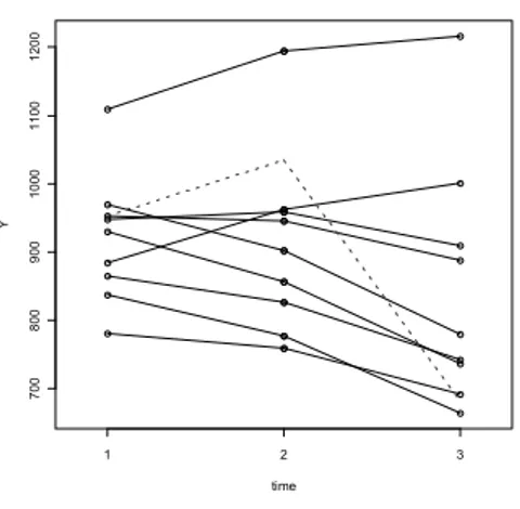
Outlier detection can be made if there is a similar behaviour among time series: in figures 1, 2 and 3 there are some examples of the concept of “similar behav-iour” for some time series considered at t 1, 2,3. In particular in figure 1 there is a quasi-linear pattern (except the dotted line segments which represent outlier data); in figure 2 there is a sort of seasonal component that increases the last value more than other two; figure 3 shows the opposite pattern. It’s important to underline that: the similar behaviour is not conditioned by the average slope of this sequence of points; the outlier is identified by a very different trajectory with respect to the other sequences of points; without other information the outlier may be every one of the three points.

time Y 1 2 3 70 0 800 900 100 0 1100 1200 1300 time Y 1 2 3 80 0 900 1000 1100 1200 1300

Figure 1 – Examples of quasi-linear trend (the

dotted line segments are an outlier). Figure 2 – Examples of positive seasonal component at t=3.

As far as the last statement, in figure 4 it’s obvious that an outlier can be iden-tified on the dotted last segment with endpoint at time 8, being the only deeply decreasing observation. Supposing a quarterly period in the ten considered time series, in this figure there is a seasonal decreasing effect of stochastic process yt at

time Y 1 2 3 700 800 900 100 0 1100 1200 1 2 3 4 5 6 7 8 400 600 800 1000 1200 1400 1600 time Y 1 2 3 4 5 6 7 8 400 600 800 1000 1200 1400 1600

Figure 3 – Examples of negative seasonal

component at t=3. Figure 4 – The showed time series have a sea-sonal component at t=3 and t=7.

3. DEFINITION OF INDEXAV

The problem of describing the common pattern of the three points is solved by the creation of an index measuring a sort of distance of three points from lay-ing on the same straight line.

A first assumption is that yit  (0 i1,..., ;n t 2,...,T . This is not a serious 1) limitation because of the possibility of translating y-coordinates (if the most of yit are

positive) or changing all negative signs in positive ones. The proof that these trans-lations don’t change too much outlier detection is provided at section 6.1.

time Y 1 2 3 0 123 4 A1y1 B2y2 C3y3 D E F time Y 1 2 3 0 246 8 A1y1 B2y2 C3y3 D E F

Figure 5 – Negative value of index AVit . Figure 6 – Positive value of index AVit .

According to figures 5 and 6, the numerator of index AVi2 is taken as double

A and C, displayed as _2, 1 3

2

i i

y y

D_  _

  . Both y-coordinates of D and B can be normalized dividing them by the sum of the three y-coordinates of A, B and C. By mean of trivial geometric evidences it’s easy to conclude that the absolute value of the numerator of AVi2 represents the length of segments FC AE

and twice the length of BD in figures 5 and 6.

Setting Si  yi1 yi2 y i3 , the index can be written:

2 1 3 2 100 (2 ) 2 S i i i i i y y y AV S      (1)

This expression, however, is too influenced by low values of Si, so that little

variations of y may identify an outlier where there is none. An alternative could be: 2 1 3 2 100 (2 ) 2 median ( ) m i i i i j j y y y AV S      (2)

Also this version of index AV is too conservative towards large values of Si.

At the end the best formulation is the following compromise solution:

2 1 3 2 100 (2 ) median ( ) i i i i j j j y y y AV S S      (3)

If y  and _i1 0 y  and _i2 0 y  then _i3 0 AV _i2 200 if median ( )_j S_j  , S_i

else AV  if _i2 0 median ( )_j S_j  ; if S_i y  and _i1 0 y  and _i2 0 y  then _i3 0

2 100

i

AV   if median ( )_j S_j  , else S_i AV  if median( )_i2 0 S_j  . S_i

So index AVi2 is zero if points A, B and C are collinear ones, while in general

AVi2 is delimited as: 100AVi2200.

Negative values of index AVi2 describe a situation similar to that repre-

sented by figure 5, while positive ones are similar to that represented by figure 6.

In these figures it is easy to see that the absolute value of AVi2 numerator is

the same, except for a scale factor, if you are considering anyone of the three dif-ferent lines laying on AC or AB or BC and try to measure the distance in term of

y-coordinates from the remaining point (respectively B, C and A). In particular

the last two have an absolute measure (segments AE and CF) that doubles the first (segment BD). However measure of AV regards point B and so sensitiveness of other two points A and C is exactly the half of point B.

time Y 1 2 3 0 5 00 1000 1500 2000 2500 2 4 6 8 10 -1 .5 -1 .0 -0 .5 0 .0 0 .5 time series AV

Figure 7 – Example of ten approximately

lin-ear time series at time 1, 2 and 3. Figure 8 – Values of index AVAVSit (dotted line) and AVmit (dashed line). it (solid line)

An example of application of (1), (2) and (3) for ten time series, showed in fig-ure 7, gives as result figfig-ure 8 and table 1. The series for i=1 is an example of how a large value of Si with respect to the medianj(Sj) gives AVim2  AVi2  AViS2 .

Instead the series i=10 has S10 that is small in respect the median(Sj) and

the index AVSi2 is, in absolute value, bigger than AVi2 and gives

2 2 2

m S

i i i

AV  AV  AV .

At the end AVi2 gives reasonable values: not too large, in absolute value, either

for small Si or for large Si.

TABLE 1

Data of example in figure 7 and 8

Data and indexes

Series i yi1 yi2 yi3 Si 2yi2-yi1-yi3 AVi2 AVSi2 AVmi2 1 2,543.2 2,506.2 2,436.6 7,485.9 69.6 0.305 0.218 0.509 2 973.7 1,012.0 1,041.0 3,026.6 -29.0 0.150 0.154 0.146 3 1,107.0 1,081.2 1,053.4 3,241.6 27.9 0.033 0.033 0.034 4 1,093.4 1,151.3 1,202.3 3,447.0 -50.9 0.106 0.102 0.110 5 1,088.2 1,003.3 923.3 3,014.8 80.0 -0.079 -0.082 -0.077 6 1,087.6 1,075.1 1,034.3 3,197.1 40.8 0.443 0.444 0.443 7 1,064.1 1,161.4 1,261.1 3,486.5 -99.7 -0.036 -0.035 -0.038 8 988.7 1,061.7 1,157.3 3,207.6 -95.6 -0.352 -0.352 -0.352 9 968.9 1,057.3 1,119.9 3,146.1 -62.6 0.407 0.410 0.403 10 213.4 148.2 97.0 458.6 51.2 -0.383 -1.530 -0.219 median 3,202.3 0,070 0.068 0.072 MAD (median absolute deviation) 269.3 0.285 0.222 0.326

4. IID TEST APPLIED TO AV INDEX SIMULATIONS

The new index AVit has an unknown distribution. What you know is that an

absolute large value of AVit, distinct from other n-1 values, is a sign of outlier

oc-currence.

In order to apply any non parametric test to the n obtained values there are two hypothesis to verify: the first one regards AVit, having the same distribution

for every i (AVit AVjt,i j, 1,..., )n , the second about independence of data (i.i.d.-independent and identical distributed variables).

The only way is to use some general simulations. A simple test to apply is pro-vided by the R-language function iid.test(), described by Benestad (2004).

Simulations of index AVit were made in different shapes and for hundreds of

time series. One of these simulations is presented as an example. In other simula-tions i.i.d. hypothesis is almost always verified.

The timing of the events can be seen in figure 9, which shows the timing of re-cord events found when time runs forwards and backwards in time. In particular there no tendency of clustering of records suggesting consistency of data with i.i.d. null-hypothesis. 0 20 40 60 80 100 05 0 10 0 15 0 20 0 iid-test time lo ca tio n 0 20 40 60 80 100

Figure 9 – Timing of the records events.

In figure 10 empirical estimates are obtained for the expectation value En (ratio

between observations exceeding the maximum of preceding observations N and

N itself) of numbers of new parallel records seen at the n-th observation for a set

of 100x100 independent series, and these estimates are compared with the ex-pected number of record-events. The empirical simulated estimates appear to fol-low the expected values.

0 20 40 60 80 100 0. 00 .20 .40 .6 0. 81 .0

Observed & Expected record-occurence

95% Confidence interval from binomial distribution Time re co rd -d en si ty

Figure 10 – Empirical estimates for the expectation value En.

0 20 40 60 80 100 05 0 10 0 15 0

Observed & Expected number of record-events

Shaded region= 95% conf.int. from Monte-Carlo with N= 200 Time e xp ( c ums u m ( 1/ (1 :n )) ) 0 20 40 60 80 100 13 4 5 Theoretical Forward Backward

Figure 11 – Relationship between the theoretical and empirical data in log-relations.

This relationship was confirmed by figure 11, in which relationship between empirical simulated data and theory can be scrutinised in more detail, showing that empirical data are likely to lie on a straight line as a good fit would do.

5. NON PARAMETRIC TEST ON AV INDEX FOR OUTLIER DETECTION

If the assumption of i.i.d. for AVit AV – as it were a unique random

vari-able – is true, with independent originated data, then the “Median Absolute procedure” of Sprent (1998) – Soliani (2005) – is “a simple and reasonable robust test” to verify for the n data ^

it

AV _{(i1,..., ;n t t} *_{), obtained from the random variables AV}

it:

0 it

1 it

H : no ^ is an outlier H : at least one ^ is an outlier

AV

AV

  

You have to calculate the following Sprent test:

^ _{median (} ^₎ . it it j jt t AV AV test AV MAD   (4)

in which you have to verify if test AV  , and where . _it 5

^ ^

median median ( )

t i it j jt

MAD  AV  AV (5)

Sprent e Smeeton (2001) say that “the choice of 5 as a critical value is motivated by the

reasoning that if the observations other than outliers have an approximately normal distribution, it picks up as an outlier any observations more than about three standard deviation from the means”.

The Chebyshev inequality is adopted because normal distribution is not so common to find out for values AV^it: it’s more likely to find a sort of delimited

asymmetric distribution. So if X is a random variable with finite second moment, then for every k>1 it’s verified that:

2 1 Pr{X E( ) }X k k     where   var( ) X (6)

This inequality permits to find out the p-value upper limit, αoss,it:

2 ^ ^ j , median ( ) 1 it it oss it t AV AV MAD          (7) In particular if test AV  then . _it 5 _{oss it,} is equal to 0.04 (4 per cent) while if

10 

it

test then oss it, is equal to 0.01 (1 per cent), suggesting that for a value of testit between 0 and 5 the H0 hypothesis is verified, while if test AV . _it 10, H0 is

not true with a p-value lower than 1 per cent. Values between 5 and 10 are to be examined accurately.

6. HOW DOES TEST.AV WORK UNDER PARTICULAR CONDITIONS

In order to evaluate goodness of this “washer” methodology in finding outliers it will be verified if an outlier originated from distribution of yi t, 1 ,yi t, ,yi t, 1

data (for simplicity y1, y2 and y3 ) is recognized by test.AV.

AV distribution depends on a 3-dimension unknown random variable

1 2 3

( ,y y y . By mean of Taylor decomposition, if you know the means , )

1 2 3

( ,  , ) and the covariance matrix ([ ]σ for ,_ij i j 1, 2,3) of ( ,y y y1 2, 3), you

can approximate mean (_AV ) and variance (_AV) of AV as it is expressed in (3). A simplifying hypothesis may be that of independence between ( ,y y y _{1 2}, ₃) (_ij  for i0  with ,j i j 1, 2,3); same unitary variance (1122 33 ); 1

median values of (y1 y2 y3) equals to mean values.

2 1 3 2 1 3 2 ( ) mean( ) 2[ ( )] AV AV              (8) 2 2 2 1 3 2 2 2 3 3 2 ( ) var( ) 2 [ ( )] AV AV                (9)

From (4) assigning test AV  . 5

sup 1 3 2 ( ) (1 10 2 ) 2 (1 5 ) AV AV AV AV y y y             (10) inf 1 3 2 ( ) (1 10 2 ) 2 (1 5 ) AV AV AV AV y y y             (11)

So you can calculate values of superior (y2sup)or inferior limit (y2inf) for y2 at

every occurrence.

By mean of simulations – keeping previous simplified hypothesis - from these last equations (10) and (11) it’s possible to verify that if ( ,₁ ₃) is similar to 2µ2, than upper/lower limit for y2 is on average of ±6.1. That is if absolute value

of y2 exceeds 6.1 times sigma than test.AV is, in general, greater of 5. This value

assures that only very atypical data are identified as outlier. 6.1. Translations

A translation of yit (i1,..., ;n t1, 2,3) makes it possible to avoid combination

of positive and negative values for y. The problem is to determine the impact of translation on test.AV. In general the impact is reductive on the number of out-liers because new values of test.AV calculated on translated yit tend to be smaller

than the one coming from original yit. So some values of test.AV near 5 could be

transformed to values smaller than 5 losing some outliers, while the impact on

AV is greater (about the same one regarding yit).

By the use of simulations the resulting rule of thumb seems to be that of not increasing y more than half the median of all y. Doing so in general test.AV de-creases of about 10 per cent.

For example if median of all yit is about 500, adding 250 to all yit, then test.AV

decreases from 6.0 to 5.4 that is also greater than 5.

The most important fact is that translation is no way a manner to lose outlier when test.AV is near 10 and translation is fewer than 50 per cent of median (i y . it)

Another example of translation is implemented in a following real application of washer (paragraph 7.2).

6.2. Applicability conditions

Index AV must have a MADt value that shouldn’t be greater than the distance

of median of AV from extreme values -100 and +200 of AV itself, when multi-plied by 5.

For example if you consider a distribution for ( ,y y y where 1 2, 3)

Uniform(0,1)

i

y  and yi are i.i.d. for i 1, 2,3, then a simulation of AV gives

MAD about 26.3 and median about zero, while five times MAD is about 131.6. It’s obvious that the distribution of AV is not informative so the pattern de-scribed by ( ,y y y is so random that to find outliers is almost impossible. 1 2, 3)

In order to give a tool for measuring a sort of informative power of AV it may be considered the following index called “madindext” expressed in percentage

values: MAD 100 15 t t madindex   (11)

This index is constructed with the “rule of thumb”. Considering a range of 300 for AV, it seems hard to find outliers when MAD >15. In fact, using formula (4),

AV is anomalous if |AV|>75, assuming for simplicity the median (AV )=0.

Test applicability is more likely, by experience, if MAD <15 and madindex <50. Table 2 makes a summary of possible scenarios.

TABLE 2

Admissible values of “madindext” for test.AV applicability

madindext possible values

madindext TEST APPLICABILITY

(0; 50] YES

(50; 100] UNCERTAIN

6.3. What about n?

Bootstrap simulations reveal that n must be at least 20-25 units to make a minimum reliable estimation of MAD(AV). The best is having n over 50 units. In the simulation below a bootstrap of 999 samples were extracted by cal-culating MAD(AV) at 95 per cent confidence levels varying n between 5 and 100, where (y1 a 1,y2  a b 2,y3 a 2b  , 3 s) i Normal(0,  , 1)

Normal( 1000, 100)

a    , Uniform( 100;100)b   and

/10 Normal( 0, 10)

s a     for (i 1, 2,3).

In figure 12 you can see convergence of MAD to 2.4 by increasing n from 5 to 100, while in figure 13 the focus is on the decreasing difference between upper limit and lower limit of the confidence interval.

0 20 40 60 80 100 2. 2 2. 4 2. 6 2. 8 3. 0 n 95-conf idence i n te rv al s m a d 0 20 40 60 80 100 0. 0 0. 1 0. 2 0. 3 0. 4 n upper -l ow er li m its 95-ci

Figure 12 – Bootstrap estimation of MAD with

samples of n between 5 and 100 units: boot-strap estimated 95% confidence intervals.

Figure 13 – The same of figure 12: upper

limit minus lower limit of 95% confidence intervals.

In figure 13 you can see that convergence of MAD can start at least from 20 hence after.

7. WASHER IMPLEMENTATIONS

7.1. Simulation

The simulation is obtained with ( ,y y y1 2, 3) where y1Normal(160, 1),

2 Normal( 200, 1)

y     , and y3 Normal(500,  , and y1) i are i.i.d.

for 1, 2,3i  . Simulation for n=1 million units give the distribution showed in figure 14 and 15 for index AV(y) and test.AV(y) respectively.

In particular mean(AV y is equal to –1.318452 and standard deviation of ( )) (AV(y)) is equal to 0.01243056. Using formula (9) the approximation of standard deviation gives the value 0.01242351 that is quite similar to the previous one.

Also median(AV y  ( )) 1.318477 and MAD(AV y ( )) 0.0124429 demon-strating that this expression, being here no outlier, is a good approximation of standard deviation. MAX(AV y  ( )) 1.257769 and MIN(AV y  ( )) 1.386591 because the simulation regards “short” time series with negative behaviour in the sense of figure 2. At last MAX(test AV . ) 4.816023 and

7

MIN(test AV. ) 3.80621 10   the absence of outlier gives very little probability of finding values greater than 5 for test.AV. As far as it regards madindex is equal to 0.0082952, that is a very small value because of the construction of series with a standard deviation equal to 1.

Histogram of AV(y) AV(y) F requ enc y -1.38 -1.36 -1.34 -1.32 -1.30 -1.28 -1.26 0 50000 100000 150000 Histogram of test.AV(y) test.AV(y) F requ enc y 0 1 2 3 4 5 0 50000 100000 150000

Figure 14 – Distribution of AV(y) for n=106_{. Figure 15 – Distribution of test.AV(y).}

7.2. Swedish municipalities between 1979 and 1987: an actual example

The washer method – by mean of washer.AV() R-function in Appendix – is

implemented using data from Dahlberg and Johanssen (2000) about Municipal Expenditure Data representing a panel of 265 Swedish municipalities over the pe-riod 1979-1987, for a total of 2,385 observations.

In the first column of a structured table the following three variables are: expend (Expediture); revenue (Revenue from taxes and fees); grants (Grants from Central

Government). In the second one there are years from 1979 to 1987 and in the third

one the number that identifies a certain municipality (id). The last column repre-sents the amounts (money per capita) as described in Dahlberg and Johanssen (2000).

First of all a value of n = 256 and a madindex less than 15.26 per cent gives rea-sonable certainty that the analysis is good enough for all years and every considered phenomenon. The greatest value of test.AV is 17.7 in the first row of Table 3, in which possible outliers with test.AV greater than 8 are collected. The total number of rows are 5,565 and only the three values of test.AV showed in table 2 are greater than 10 (42 rows, of which 38 are omitted, enclose test.AV between 5 and 10).

TABLE 3

Output of washer.AV() for Dahlberg and Johanssen (2000) data

Data, factors and indexes

phen. t2 series y1 y2 y3 test _AV AV n median _AV MAD _AV madindex _(%)

grants 1981 2184 0.0051 0.0016 0.0057 17.72 -28.60 265 0.0335 1.6161 10.7740 grants 1982 2184 0.0016 0.0057 0.0054 11.09 16.24 265 0.3561 1.4322 9.5481 expend 1986 1165 0.0157 0.0239 0.0179 10.67 12.81 265 -0.1907 1.2180 8.1201 grants 1986 2506 0.0084 0.0064 0.0100 9.81 -14.15 265 -0.7701 1.3647 9.0982 revenue 1982 1643 0.0115 0.0231 0.0123 9.45 25.62 265 3.9927 2.2885 15.2564 revenue 1986 1165 0.0113 0.0198 0.0123 9.19 19.89 265 0.1960 2.1442 14.2946 grants 1980 2184 0.0047 0.0051 0.0016 8.83 15.39 265 0.4208 1.6960 11.3064

Note: t2 is the time reference of y2

Looking at figure 14 it’s obvious that year 1981, for municipality number 2184, presents an anomalous value of grant. The outlier is so intensive that even the three values with 1982 in the middle present anomalies. The simple graphical analysis – in figure 15 – of expend time series of municipality number 1165 is not so obvious. It’s not trivial that expenses of year 1986 are an outlier as reported by

washer.AV function in table 3. It is necessary the “washer” comparison with other

time series to deduce the final result.

1980 1982 1984 1986 0. 000 0. 001 0. 0 02 0. 003 0. 004 0. 005 0. 006 years Y 1979 1980 1981 1982 1983 1984 1985 1986 1987 1980 1982 1984 1986 0. 000 0. 001 0. 0 02 0. 003 0. 004 0. 005 0. 006 years Y 1979 1980 1981 1982 1983 1984 1985 1986 1987

Figure 14 – Time series of municipality

num-ber 2184.

Figure 15 – Time series of municipality

num-ber 1165.

As it was mentioned before in paragraph 6.1 an example of translation was im-plemented to “grant” data. The median of y was about 0.005 and so data was augmented of 0.0025 so that increment was about 50 per cent on y values. While the first row of table 2 shows a test.AV equal to 17.72 the transformed y give 17.53 that is about 1 per cent smaller than the previous one. The impact is greater on other y: madindex decreases of about 35 per cent from 10.77 to 6.99 because translation reduces variability of index AV.

8. CONCLUSIONS

After the identification of time series with similar behaviour - as explained at the beginning of the work - the implementation of washer method to detect out-lier - using R-language function washer.AV() available in the Appendix - needs

a step by step procedure:

1) The data set {ypit} (where p1,...,P; i1,...,n; t 1,...,T; n 20 25 ; 3

T  ), made of positive values, is organized as a longitudinal table (that one

of relational data bases) with classification attributes p, i and t respectively on columns 1, 3 and 2, while positive values are recorded in column 4. In the example of pollution recorder machines column 1 attribute regards the type of recorded pollution (phenomena), column 2 contains record time (time), column 3 the identification of the machine (i-th series), while column 4 is for values of polluter (y). Missing values are treated by dropping

, , 1 , , , , 1

(yp i t ,yp i t,yp i t ) if at least one of the three is a missing value.

2) After implementation the resulting data frame in output has to be controlled to verify if any i-th series gives values of madindex.AV greater than 50 per cent to know that they cannot be tested because washer method is hardly applicable. 3) Outlier detection regards in particular the central observation but also other

points are monitored. To verify the last observation you need to keep in mind that test sensitiveness is halved: if the last value is an outlier, a test value of about 5 is comparable to 10 for an outlier in the central position.

4) Values of test.AV greater than 10 reveal almost certainly an outlier while lower values of test.AV but greater than 5 are to be evaluated one by one.

The implementation of washer method to detect outliers provides a new out-lier detection methodology that is efficient for time-saving elaboration and im-plementation procedures, adaptable for general assumptions about distribution of time series whose requested length is really a minimum, reliable and effective as involving robust non parametric test.

Further applications of the index AV can be found using median and MAD of index AV from a descriptive point of view.

Divisione Analisi e ricerca economica territoriale ANDREA VENTURINI1

Banca d’Italia – Sede di Venezia

ACKNOWLEDGMENTS

I would like to thank my wife Kikki for her patience, Vanni Mengotto for encourage-ment and useful suggestions, Mauro De Angelis for interesting observations, Elena Mattevo and Andrea Petrella for lexical suggestions, and an anonymous reviewer of Bank of Italy whose remarks and suggestions have improved this work. In memory of my fa-ther Francesco, who I thank every day of my life.

1 _{The views expressed are those of the author and do not involve the responsibility of the Bank}

of Italy. Usual disclaimers apply.

Regional Economic Research Division - Venezia Branch of Bank of Italy - San Marco, 4799/a - 30124 Venezia (Italy) - Tel. +390412709252 Fax +390415200791 andrea.venturini@bancaditalia.it.

APPENDIX

############################################################################################### ## Function washer.AV in R-language (R version 2.8.1 or more recent)

## V. 1.0 June 2010

## Author : Andrea Venturini (andrea.venturini@bancaditalia.it)

## Disclaimer: THE PROGRAM IS PROVIDED "AS IS", WITHOUT WARRANTY OF ANY KIND, EXPRESS OR IMPLIED, INCLUDING BUT NOT LIMITED TO THE ## WARRANTIES OF MERCHANTABILITY, FITNESS FOR A PARTICULAR PURPOSE AND NONINFRINGEMENT. IN NO EVENT SHALL THE AUTHOR BE LIABLE FOR ANY CLAIM, ## DAMAGES OR OTHER LIABILITY, WHETHER IN AN ACTION OF CONTRACT, TORT OR OTHERWISE, ARISING FROM, OUT OF OR IN CONNECTION WITH THE PROGRAM OR ## THE USE OR OTHER DEALINGS IN THE PROGRAM.

################################################################################################ washer.AV = function( dati ) # p t i y

{ # dati structure: phenom./date/series/values/... other # example: Phenomenon Time Zone Value ... # --- --- -- --- --- # Temperature 20091231 A1 20.1 ... # Temperature 20091231 A2 21.0 ... # ... # Rain 20081231 B1 123.0 ... # ... ############################################################################################### AV = function(y) { # y matrix 3 columns (y1 y2 y3) and n rows

AV=array(0,length(y[,1]))

100*(2*y[,2]-y[,1]-y[,3])/(median(y[,1]+y[,2]+y[,3])+ y[,1]+y[,2]+y[,3]) } # output array AV

############################################################################################### test.AV = function(AV) { # AV array n rows

t(rbind(test.AV=abs(AV-median(AV))/mad(AV),AV=AV,n=length(AV),median.AV=median(AV),mad.AV=mad(AV) , madindex.AV=mad(AV)*1000/150 )) }

# col 1 2 3 5 6 7 # output: test / AV / n / median(AV) / mad(AV) / madindex

################################################################################################ if (min(dati[,4])> 0) { dati=dati[which(!is.na(dati[,4])),] dati=dati[order(dati[,1],dati[,3],dati[,2]),] fen=rownames( table(dati[,1]) ) nfen=length(fen) out= NA for ( fi in 1:nfen) { print(c("phenomenon:",fi),quote=FALSE) time=rownames( table(dati[which(fen[fi]==dati[,1]),2]) ) n=length(time) for ( i in 2:(n-1) )

{ c1=which(as.character(dati[,2])==time[i-1] & dati[,1] == fen[fi]) c2=which(as.character(dati[,2])==time[i ] & dati[,1] == fen[fi]) c3=which(as.character(dati[,2])==time[i+1] & dati[,1] == fen[fi]) mat=matrix(0,3,max(length(c1),length(c2),length(c3))+1) if (length(c1) > 5) { j=1 for ( k in 1:length(c1) ) { mat[1,j]=c1[k] if (!is.na(match(c1[k]+1,c2))) { mat[2,j]=c1[k]+1 if(!is.na(match(c1[k]+2,c3))) {mat[3,j]=c1[k]+2 j=j+1 } } } mat=mat[,which(mat[3,]!=0)] y=cbind(dati[mat[1,],4], dati[mat[2,],4], dati[mat[3,],4]) out=rbind(out,data.frame(fen=fen[fi],t.2=time[i], series=dati[mat[2,],3],y=y,test.AV(AV(y)))) } } } rownames(out)=(1:length(out[,1])-1) washer.AV=out[2:length(out[,1]),] # col 1 2 3 4 5 6 7 8 9 10 11 12 # output: rows /time.2/series/y1/y2/y3/test(AV)/AV/ n /median(AV)/mad(AV)/madindex(AV) # end function washer.AV

} else print(" . . . zero or negative y: t r a n s l a t i o n r e q u i r e d !!!") }

REFERENCES

V. BARTNETT, T. LEWIS, (1994), Outliers in Statistical Data, John Wiley & Sons, New York.

R.E. BENESTAD(2004),Record-values, non-stationarity tests and extreme value distributions,“Global and Planetary Change”, vol. 44, issue 1-4, pp. 11-26.

M. DAHLBERG, E. JOHANSSON,(2000), An Examination of the Dynamic Behaviour of Local

Govern-ments using GMM Bootstrapping Methods,“Journal of applied econometrics”,vol 5, pp.

401-416.

L. KOVACS, D. VASS, A. VIDACS(2004),Improving Quality of Service Parameter Prediction with

Prelimi-nary Outlier Detection and Elimination,IPS’2004,Budapest Hungary.

S. PAPADIMITRIOU, H. KITAWAGA, P.B. GIBBONS, C. FALOUTSAY,(2002), LOCI: Fast Outlier

Detec-tion Using the Local CorrelaDetec-tion Integral,Technical Report IRP-TR-02-09,Intel Research

Laboratory,Pittsburgh.

L. SOLIANI (2005), Manuale di Statistica per la Ricerca e la Professione. Statistica Univariata e Biva-

riata, Parametrica e Non-Parametrica per le Discipline Ambientali e Biologiche, Dipartimento di

Scienze Ambientali, Università di Parma.

P. SPRENT (1998) Data Driven Statistical Methods, Chapman and Hall, London.

P. SPRENT, N.C. SMEETON,(2001),Applied Nonparametric Statistical Methods (3rd ed.),Chapman and Hall, London.

SUMMARY

Time series outlier detection: a new non parametric methodology (washer)

The production and exploitation of statistical data for a large amount of high fre-quency time series must allow a timely use of data ensuring a minimum quality standard. This work provides a new outlier detection methodology (washer): efficient for time-saving elaboration and implementation procedures, adaptable for general assumptions and for needing very short time series, reliable and effective as involving robust non pa-rametric test. Some simulations, a case study and a ready-to-use R-language function (washer.AV()) conclude the work.