Study of inelastic processes in proton-proton collisions at the LHC with the TOTEM experiment

(1)

Universit`

a degli Studi di Pisa

Facolt`a di Scienze Matematiche Fisiche e Naturali

Corso di Laurea in Scienze Fisiche

Curriculum Fisica delle Interazioni Fondamentali

Tesi di Laurea Specialistica

Study of inelastic processes in proton-proton

collisions at the LHC with the TOTEM

Experiment

Relatore: Candidato:

Prof. S. Lami P. Brogi

Correlatore: Prof. G. Latino

Anno Accademico 2010/2011

(2)

(3)

Introduction

The TOTEM [1] experiment, located into the CMS cavern at the CERN Large Hadron Collider (LHC), is one of the six experiments that are investigating high en-ergy physics at this new machine. In particular TOTEM has been designed for TO-Tal cross-section, Elastic scattering and diffraction dissociation Measurements. The total proton-proton cross-section will be measured with the luminosity-independent method based on the Optical Theorem. This method will allow a precision of 1_÷2% at the center of mass energy of 14 TeV. In order to reach such a small error it is neces-sary to study the p-p elastic scattering cross-section (dσ

dt) down to |t|

1 _{∼ 10}−3 _GeV2

(to evaluate at best the extrapolation to t = 0) and, at the same time, to measure the total inelastic interaction rate. For this aim, elastically scattered protons must be detected at very small angles with respect to the beam while having the largest pos-sible η 2 _{coverage for particle detection in order to reduce losses of inelastic events.}

In addition, TOTEM will also perform studies on elastic scattering with large mo-mentum transfer and a comprehensive physics programme on diffractive processes (partly in cooperation with CMS), in order to have a deeper understanding of the proton structure.

For these purposes TOTEM consists in three different sub-detectors: two gas based telescopes (T1 and T2) for the detection of inelastic processes with a coverage

1_{In a two body scattering a + b → a + b, defining the four-momentums of ingoing (p1, p2)}

and outgoing (p3, p4) particles , the kinematics can be described using the Lorentz invariant Mandelstam Variables (s, t, u), that are defined as:

s = (p1+p2)2 _{= (p3+p4)}2

t = (p1−p3)2 _{= (p2−p4)}2

u = (p1−p4)2_{= (p2−p3)}2

Therefore s represents the square of the c.m. energy, while t is the four-momentum transfer squared.

2_{The pseudorapidity is defined as η = − ln(tan}θ

2), where θ is the polar angle of the scattered

particle with respect to the beam direction.

(8)

6 Introduction

in the range of 3.1 _{≤ |η| ≤ 6.5 on both sides of the interaction point 5 (IP5),} and silicon based detectors for the elastically scattered protons, located in special movable beampipe insertions called Roman Pots (RPs), at about 147 m and 220 m from the interaction point.

The work done by the candidate reported in this thesis mainly consists in three subjects: the tuning of the simulation for the T2 inelastic telescope, the study of the noise of the T2 detector and a preliminary study concerning the detection perfor-mance for inelastic events. In the following, the first chapter describes the TOTEM experiment and the LHC machine, with a particular attention to the T2 telescope and its analysis software, being of critical importance for the work of this thesis. The second chapter introduces the physics programme of the TOTEM experiment. Chapter three describes the tuning of Geant4 parameters and the improvement of the simulated geometry for the T2 detector, while chapter four summarizes an im-portant and demanding study on the detector noise. Finally in chapter five some preliminary studies on inelastic processes are presented, in order to show the per-spective for the TOTEM experiment to perform the measurement of the inelastic cross section in a wide kinematic range.

(9)

Chapter 1 TOTEM at the Large Hadron

Collider

The TOTEM experimental apparatus, consisting in three different sub-detectors, is located at the Interaction Point 5 (IP5) of the CERN (European Organization for Nuclear Research) Large Hadron Collider (LHC), sharing it with the CMS experi-ment. In this chapter the TOTEM detectors will be described, after a brief overview of the machine. Being the T2 inelastic telescope the main subject of this thesis work, more emphasis will be dedicated to this detector in the following.

1.1 The machine

The LHC, originally started up in September 2008, is the biggest and most powerful particle collider actually operating. It is a circular accelerator of about 27 Km of circumference, located underground (50 to 175 m) into the tunnel of its precursor LEP. It was designed in order to collide two counter rotating beams of protons or heavy ions. For proton-proton collisions it is foreseen to reach a peak luminosity up to 1034_cm−2_s−1 _{at a center of mass (C.M.) energy of 14 TeV. It is currently running}

up to 1032_cm−2_s−1 _{and at a 7 TeV C.M. energy. While the design energy is planned}

to be reached in 2014.

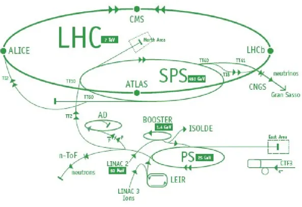
In reality LHC is the final stage of an accelerator complex (figure 1.1) located in the north-west suburbs of Geneva on the French-Swiss border. The first step of the

(10)

8 1.1 The machine

Figure 1.1: Schematic layout of the CERN accelerator complex.

chain is provided by the LINAC2 linear accelerator, where protons obtained from the dissociation of hydrogen are accelerated up to 50 MeV. They are then sent into the PS Booster that brings them up to 1.4 GeV. Then, inside the Proton Synchrotron (PS) they reach an energy of 26 GeV and are ready for the last pre-acceleration stage in the Super Proton Synchrotron (SPS) which accelerates protons up to 450 GeV before injecting them into the LHC ring. Where they are brought to the final energy (presentely 3.5 TeV per beam), before colliding in the four provided colli-sion points, where are located the six CERN experiments (ALICE, ATLAS/LHCf, CMS/TOTEM, LHCb) with their detectors.

In order to keep two counter-rotating proton beams, the machine needs two separated rings with opposite magnetic fields to bend same charge particles rotating on opposite directions. Moreover, in order to bend 7 TeV protons a magnetic field of 8.36 Tesla is required. The goal is achieved using two different superconducting dipoles housed in the same yoke, cooled down to 1.9 K with superfluid helium. The whole accelerator is composed of 1296 superconducting dipoles (bending magnets)

(11)

1.1 The machine 9

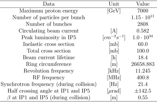
and more than 2500 other magnets used to guide and focus the beams around the ring. The main parameters of the machine are reported in table 1.1 with their nominal values [2].

Data Unit Value

Maximum proton energy [GeV] 7000

Number of particles per bunch 1.15· 1011

Number of bunches 2808

Circulating beam current [A] 0.582

Peak luminosity in IP5 [cm−2_s−1_] _1.0_{· 10}34

Inelastic cross section [mb] 60.0

Total cross section [mb] 100.0

Beam current lifetime [h] 18.4

Ring circumference [m] 26658.883

Revolution frequency [kHz] 11.245

RF frequency [MHz] 400.8

Synchrotron frequency (during collision) [Hz] 21.4 Half crossing angle at IP1 and IP5 [µrad] _±142.5 β at IP1 and IP5 (during collision) [m] 0.55

Table 1.1: Main parameters of the LHC machine at nominal c.m. energy (14 TeV). One of the most important parameters shown here is the luminosity (_L), repre-senting the factor of proportionality between the event rate R and the interaction cross-section σ:

R = Lσ

So it is easy to understand why, in order to observe phenomena with a very low cross-section, it is important to reach the highest possible luminosity, which can be defined as [3]:

L = fnb

N1N2

4πσ∗ xσy∗

In this equation σx and σy represent the transverse gaussian beam profiles at the IP

in the horizontal and vertical directions. N1, N2 represent the number of protons

in the colliding bunches, f is the frequency of revolution of bunches and nb the

number of bunches. The equation is not exact for calculating L at LHC but it means that a higher luminosity can be reached with small transverse size bunches at IP or a high number of bunches (f depends only on the accelerator length) or highly populated bunches. However anyone of these requirements can cause several

(12)

10 1.2 The TOTEM detectors

problems. Higher focussed bunches lead to severe “beam-beam effects” (when two bunches cross, the particles are deflected by the strong electromagnetic field, this deflection is stronger for denser bunches, and can lead to particle losses). Increasing the number of particles in each bunch results in more event pile-up and this is to avoid for a better understanding of the physics process. Furthermore, the bunch crossing rate is limited by the time resolution of the detectors and read-out systems employed.

1.2 The TOTEM detectors

The TOTEM experiment is composed by three different detectors: the two telescopes T1 and T2, based on CSC (Cathode Strip Chamber) and GEM (Gas Electron Mul-tiplier) technology, respectively; and the Roman Pots (RPs) equipped with silicon detectors. The three detectors are located (see figure 1.2) symmetrically on both sides of the interaction point IP5, the same shared with the CMS experiment. The telescopes are located at 9 m and 13 m from the interaction point, while the RPs are located in special vacuum insertions along the beam-pipe at 147 m and 220 m from IP5. The detectors designed for a particular purpose have a specific acceptance region; in particular the TOTEM physics programme requires a good acceptance for angles very close to the beam axis. The pseudo-rapidity coverage for T1 and T2 is 3.1 < _{|η| < 6.5, and the RPs placed inside the vacuum pipe allow the detection} of elastically scattered very close to the beam (till few µrad). The data acquisition system is designed to be compatible with CMS to have the possibility of a common data taking in order to combine TOTEM and CMS, therefore obtaining the largest acceptance (in eta) detector ever built. The two inelastic telescopes have a 2π cov-erage in φ and a good efficiency in order to minimize losses of non-diffractive and minimum bias events. They are designed to ensure the detection of about the 95% of all inelastic events having charged particles within their geometrical acceptance (about 99.5% of all non-diffractive events and 84% of all diffractive processes). Even if the telescopes are outside the central region of the CMS magnetic field and cannot provide information about the momentum of tracked particles, they are in front of

(13)

1.2 The TOTEM detectors 11

Figure 1.2: Location of the TOTEM detectors at IP5.

two CMS calorimeters, HF for T1 and Castor for T2, respectively. Therefore the combination of this two kind of detectors could permit a more complete study of the diffractive processes, low-x phenomena and particle/energy flows in the very forward region. The read-out task of all the TOTEM detectors is provided by the VFAT2 (Very Forward ATLAS and TOTEM chip) [4], a front-end ASIC (Application Spe-cific Integrated Circuit) designed in CMOS technology for the TOTEM experiment itself to process the signals and marked by trigger capability.

1.2.1 The Roman Pots

Silicon detectors are placed inside each secondary vacuum insert, called “pot”. These special pots are moved into the primary vacuum through a bellow. This device allows to physically separate the detectors from the primary vacuum, in order to preserve it from an uncontrolled out-gassing of the materials. This experimental technique is well known since it was introduced at the ISR and it has been successfully employed

(14)

Figure 1.3: Schematic view of a Roman Pot station

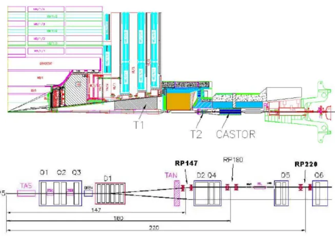
in other colliders like SppS, TEVATRON, RIHC and DESY. Moreover the use of movable inserts is useful because it allows to retract the detectors in a safe position when the beam is in an unstable condition, avoiding useless risk and exposure to radiation for the silicon detectors. There are two RP stations, like the one depicted in figure 1.3, for each side of IP5, placed at a distance of about 147 m and 220 m along the beam-pipe, symmetrically on both sides. A magnetic dipole between the two RP stations provides a magnetic spectrometer which helps proton momentum reconstruction. Each RP station is composed by two RP units (figure 1.4) separated by a distance that allows local track reconstruction and trigger selection by the track angle. A RP unit consists in 3 pots, two approaching the beam vertically and one horizontally, the scheme of silicon detectors displacement is shown in figure 1.5. This configuration was chosen to provide the best reconstruction of the fractional momentum loss (ξ) of diffractive scattered protons. Looking inside the pots at the detectors itself, these are constituted by a stack of 10 planes of silicon “edgeless” devices. These are single-sided AC p+_{-n microstrip detectors 300 µm thick with 512}

strips and a pitch of 66 µm. Half of the silicon devices have their strip oriented at an angle of +45◦, with respect to the edge facing the beam, and the others to −45◦_{. This structure allows a single hit resolution of about 20 µm. The special}

(15)

Figure 1.4: Schematic view of a Roman Pot unit.

Figure 1.5: Schematic view of the three Ro-man Pot silicon detector overlap.

edgeless technology allows to reduce the insensitive edge area to about 50 µm [5] (for the side facing the beam). This feature contributes, together with the ability of approaching the beam at about 1 mm from its axis, to the possibility to detect elastically scattered proton down to few µrad. This is important also to reduce the error in the extrapolation of the elastic cross section to the optical point t =0, and consequently the error on the total cross section measurement. Aging studies for these detectors have shown a behaviour similar to the standard silicon devices. It is expected that these detectors will be working up to an integrated luminosity of about 1 fb−1.

1.2.2 The T1 telescope

The T1 telescope has two arms, one for each side of IP5, and it is installed into the CMS End Caps at a distance of 7.5 to 10.5 m. Each arm surrounds the beam-pipe and has a coverage in pseudo-rapidity of 3.2 < _{|η| < 4.7. The detector is based on} Cathode Strip Chamber (CSC) technology, the CSC being a multi-wire proportional chamber, with a read-out made by a segmented cathode. Each plane of T1 consists in six trapezoidal CSCs. Five of these planes, equally spaced in z, build an arm of the telescope. In order to have a better pattern recognition for track reconstruction and to reduce the material concentration in front of the CMS calorimeter (Hadron Forward) the six trapezoidal CSCs of each plane are tilted with respect to each other

(16)

Full gas gap 10 mm Wire spacing 3 mm Wire diameter 30 µm

Strip pitch 5 mm Strip width 4.5 mm Chamber thickness 43 mm

Table 1.2: Basic parameters of T1 Chathode Strip Chambers

by a small angle varying from ₋₆◦ _{to +6}◦ _{in steps of 3}◦_{. The read-out boards on}

both sides of a chamber are segmented in strips and are rotated to +60◦ and −60◦

with respect to the anode wires. That allows (according to beam test studies) a spatial resolution of about 0.8 mm, when using a digital read-out. Moreover the gas mixture employed is Ar/CO2/CF4 in a ratio 40%/50%/10%, and with this kind

of mixture and a gas gap of 10.0 mm the time response for this detector (even if inherently slow) is compatible with the rates required by TOTEM. Aging studies for this detector have shown no loss of performance after an irradiation equivalent to a total charge integrated on the anode wire of 0.065 C/cm, which corresponds to 5 years of running at a luminosity of 1030_cm−2_s−1_{. In table 1.2 are summarized}

some important parameters of the T1 Cathode Strip Chambers, and in figure 1.6 are shown an arm of T1 (left) and a schematic view of one chamber of the telescope (right).

Figure 1.6: Left: a T1 telescope arm. Right: schematic view of anodic wires and cathodic

(17)

Figure 1.7: Schematic view of one plane of the T2 detector.

1.2.3 The T2 telescope

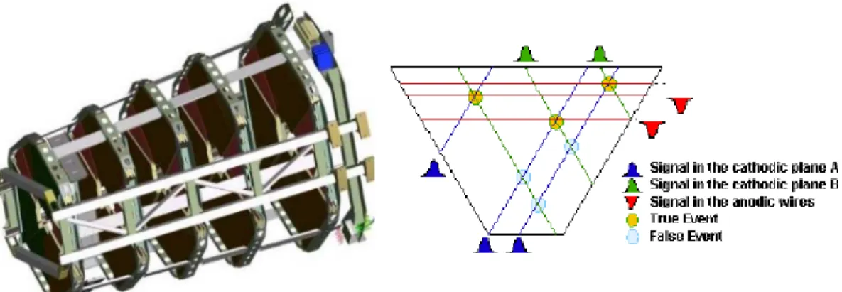
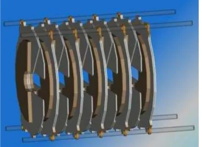
The T2 telescope is composed by 40 planes of Gas Electron Multiplier (GEM) de-tectors, with an angular coverage of 192◦ _{each. The schematics of one of this plane}

is shown in figure 1.7; it displays the detailed shape that allows the detector to enclose the beam-pipe at its center. Moreover, cooling and read-out sectors are also visible in the picture. One quarter of the telescope is made by 10 planes aligned and assembled back-to-back in five pairs, each distant 91.0 mm from the other, for a total length of the quarter of about 40 cm (supports excluded). Two quarters form an arm of the telescope with a coverage of 360◦ _{in φ and an overlap region of 12}◦_,

to minimize the edge inefficiency. The two arms are placed on each side of IP5 lo-cated at_{±13.5 m inside the shielding behind HF and before the Castor calorimeter.} More precisely, the Z position of the first GEM plane with respect to the IP is 13.83 m. From figure 1.8 it is possible to evaluate the T2 position with respect to the CMS calorimeters and the ion pump station placed in the beam-pipe, just in front of the T2 telescope. Moreover in figure 1.9 a 3D schematic view of one arm of the T2 detector is shown. The T2 coverage in pseudo-rapidity is 5.3 ≤ |η| ≤ 6.5, the resolution in η is good, down to 0.04, and it allows a good capability in

(18)

discriminat-16 1.2 The TOTEM detectors

Figure 1.8: Location of one arm of the T2 detector inside the shielding behind HF, in front of the Castor calorimeter.

(19)

ing against beam-gas background and secondary particles produced in interactions with the beam pipe. The GEM technology used for the T2 telescope ensures a high rate capability, good spatial resolution and good radiation hardness. This kind of detectors, invented about a decade ago by Fabio Sauli [6], are characterized by a very high efficiency in detecting charged particles and they are used also in other CERN experiments like COMPASS and LHCb.

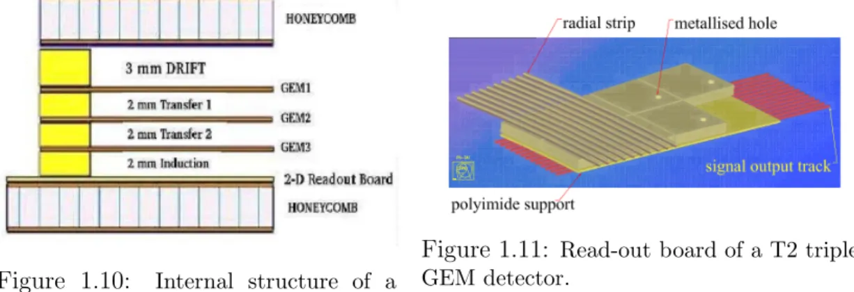
The structure of the GEM chambers is based on the “triple-GEM” scheme adapted also in COMPASS, in which three GEM foils are assembled in cascade, as shown in figure 1.10, where the transversal view displays the composition of a semicircular detector, made by a stack of three GEM foils, separated by 2 mm insu-lator spacers and mounted on the honeycomb supports. This configuration is useful in order to obtain an high gain reducing the discharge probability (below 10−12). A

Figure 1.10: Internal structure of a

triple-GEM detector.

Figure 1.11: Read-out board of a T2 triple-GEM detector.

GEM foil is composed by a 50 µm polyimide sheet coated with 5 µm copper on both sides. On the foil there is a high density of holes, obtained by a photo-lithographic method, with a double conical shape (the distance between the holes is 140 µm). The diameter of the holes is 65 µm in the middle of the GEM foil and 80 µm at the surface. A charged particle crossing the chamber ionizes the gas that fills the drift volume (a mixture of Ar/CO2 at 70%/30%) producing primary electrons, which are carried by

an electric field of about 2.4 KV/cm towards the holes of the top GEM-plane, where an electric field of about 50 KV/cm, which generates the electron multiplication, is present. This field is achieved by applying a voltage (about 400V) between the two copper layers of a foil. For this configuration the factor of multiplication is about

(20)

18

1.3 TOTEM offline software and T2 reconstruction chain 20 and the electrons produced inside the channels were driven by a field of about 3.6 KV/cm through the transfer zone to the next GEM planes (where the following electron multiplications happen) till finally the charge is collected on the read-out board. This board was specifically designed for TOTEM, and it has an inner radius of 42.46 mm and an outer radius of 144.46 mm. The structure as shown in figure 1.11 is composed by two layers of 15 µm copper, separated by a polyimide foil of 50 µm. The two layers have different patterns, one is divided in strips while the other in pads. The first is divided in 2 sectors of 256 concentric circular strips, 80 µm wide and with a pitch of 400 µm. Each sector covers an azimuthal angle of 96◦ _and

the strip segmentation allows track radial reconstruction. The second layer instead is segmented in pads, which provide level-1 trigger information and track azimuthal angle reconstruction. The pads form a matrix of 24x65 elements, varying in size from 2 x 2 mm2 _{to 7 x 7 mm}2_{, in order to have a constant ∆η x ∆φ} _{∼ 0.06 x 0.05}

rad. Beam tests on detectors have shown a spatial resolution in radial coordinates of about 100 µm (with digital VFAT read-out), while the time resolution achievable with the electric field reported above is about 18/20 ns. Concerning the detector aging, tests on COMPASS triple-GEMs have shown that a charge up to 20 mC/mm2

can be integrated on the read-out board without major effects. This corresponds to running for at least 1 year at luminosities of 1033_cm−2_s−1 _{. All these features make}

the triple-GEM technology a proper choice for the T2 telescope requirements.

1.3 TOTEM offline software and T2

reconstruction chain

Since the use of the TOTEM offline software is mandatory for the thesis work, in this section a brief description of this tool is provided. Particular attention has been paid to the T2 reconstruction chain, since it is fundamental, to understand this thesis work, to know how the particle induced signals (real or simulated ones) collected by the detector are treated at the analysis level to reconstruct useful observables like: clusters, hits and tracks.

(21)

1.3 TOTEM offline software and T2

reconstruction chain 19

Looking at the software structure, TOTEM is using a C++ based framework developed by the CMS experiment (CMSSW) [7]. This allows to reconstruct and record physics and simulation events ensuring a full compatibility of TOTEM and CMS data processing in future analyses studies. This framework consists of an Event Data Model (EDM), services needed by the simulation and reconstruction modules that process event data. The EDM is based around the concept of an Event. This is a C++ object container for all the information coming from real data acquisition or from physical process simulation. The Event starts as a collection of raw data (signals) from detectors or as a collection of the generated particles in a Monte Carlo (MC) simulated event. Then during the processing (via reconstruction modules) the Event is used to pass the data from one module to the next, to access them and to store the products of processing in objects. All these objects contained in the Event may be stored (collectively or individually) in ROOT format files, and are thus directly readable in ROOT [8].

Effectively once that one has a data file, from a real detector acquisition or the simulation of a physical process, the interesting observables can be reconstructed on it and then an analysis on these observables can be performed. The reconstruction is identical for both real data and simulated processes, and is performed for the T2 detector in four main steps: clusterization, hit reconstruction, road finding and tracking [9]. Anyway if one wants to simulate the detector response for a physical process there are three steps to do before the reconstruction; since the simulated event has to be generated, propagated and digitized. Because of the importance of the simulation in our thesis work, we spend few words also in the description of these steps. The event generation is handled by a Monte-Carlo generator: Pythia6 [10], Pythia8 [11] and Phojet [12] are common ones and are all used in this thesis. These generators allow to produce the final state of a proton-proton collision for a wide variety of physical processes (and C.M. energies). Moreover there is also the possibility to use a Particle Gun, that allows to generate single or multiple particles with fixed (or alternatively flat distributed) values of η,φ and energy at the IP. After the generation of the physical process, it has to be propagated from the IP to the detectors, simulating the interaction of the particles with matter as

(22)

20

1.3 TOTEM offline software and T2 reconstruction chain well as the effect of the magnetic field. This is performed by a software tool named Geant4 [13] (a more comprehensive description on it is reported in section 3.1). Given the Geant4 simulation of particle entry and exit points in the detector active volumes and their energy deposition, the digitization step reproduces the electrical response of the detector itself (for instance of a T2 GEM chamber). For what concerns the T2 triple GEM detectors, the proper module inside CMSSW is able to reproduce the digital output signal of the chambers. So, the outputs of the digitization are the pad/strip digital status (ON/OFF) for each telescope plane. This is the same kind of output given by a real data acquisition and it provides the input for the reconstruction process. The first reconstruction step is the clusterization. Since a particle traversing a detector device typically turns ON more than one read-out channel, it’s important to collect all the neighbouring pad/strips in an unique pad/strip cluster. The clusterization algorithm manages to do that and saves all the cluster information that could be useful for the next steps or for analysis purposes. For what concerns pad clusters, only the active pad that touches each other via a side were considered neighbouring and collected in a cluster, while the pad that touches each other via a corner were reconstructed as two different clusters. The most important information saved for each cluster are: the detector ID to which the cluster belongs; the position of the cluster itself, the cluster type (pad or strip) and the cluster size (number of pads/strips in the cluster). The detector ID is an integer number that permits to identify to which plane and quarter of the T2 detector the cluster belongs.

At this point it could be useful to explain the numeration scheme used to identify the T2 detector components. The T2 quarters are numbered from 0 to 3, and are called H0, H1, H2 and H3. H0 is the plus near quarter of the detector, H1 is the plus far, H2 the minus near and H3 the minus far. Near and far means respectively that the quarter is located in the inner side of the LHC ring or in the outer side. While plus and minus means that the quarter is located respectively on the positive half-line of the Z axis1 _{or on the negative one. The planes of each quarters are then}

1_{The coordinate system we usually refer to in this thesis work has the origin in IP5, the X axis}

pointing toward the center of the LHC ring, the Y axis pointing to the ground surface and the Z axis along the beam line.

(23)

numbered from 0 to 9 starting from the plane nearest to IP5 that is number 0, from the farthest one that is number 9.

After this little digression on the numbering scheme we restart to describe the reconstruction chain, from the hit reconstruction, that is the next step after the clusterization. In fact most of the times that a ionising particle crosses a detector plane it generates both a strip and a pad cluster. For this reason the hit recon-struction algorithm matches the overlapping pad and strip cluster to form a class 1 hit. While the clusters that don’t match with any others are called class 2 hits and become equally part of the hit collection. Then all the information related to an hit are saved in appropriate objects, the most important ones being: the hit position (and resolution on it), the hit class (1 ot 2), the composition of a class 2 hit (strip or pad) and all the information inherited by the clusters that composed the hit itself. In the case of a class 1 hit the position information are reconstructed taking advantage from both pad cluster and strip cluster, because the pad cluster has a better angular resolution and the strip cluster a better radial one. This allows to have a more precise measure of the real particle position.

Achieved this step we want to reconstruct also the track (3D straight line) that the particle follows inside the detector. We do this in two distinct steps; we first search for all the “roads” and then we make a linear fitting on these roads to find the tracks. A road is a collection of hits on different planes that are roughly aligned. A road finding algorithm is used, that acts in a few consecutive levels. This algorithm works quarter by quarter and at first level considers only the pad clusters, because of their better granularity and efficiency. At this level starting from the first detector plane (nearest to IP) for each cluster in this plane it computes a raw track with all the clusters in the second plane. After the algorithm checks for each raw track if there is a cluster in the third plane in a position compatible with the crossing point of the raw track in this plane. Compatible means that the center of the pad cluster is more than 2σ closer to the crossing-point of the track. If there is a such cluster in the third plane this is associated to the other two to form the road, then the search for clusters continues in the next planes and when a compatible one is found it is associated to an existing road. Otherwise the algorithm searches for clusters

(24)

22

1.3 TOTEM offline software and T2 reconstruction chain compatible with the raw track for other two planes (i.e. fourth and fifth), and if there aren’t none this possible road is discarded and the search for the next starts with a different raw track. After that for the first plane all the possible roads has been computed, the algorithm moves to the second plane and follows the same procedure but using only the pad cluster still not belonging to any road. And so on, until the last plane. In these further steps, in which the algorithm computes the road starting not from the first plane, it also searches back for clusters to associate to the road in the planes that precede the starting one and not only in the plane that follows it. Once that all these pad cluster collections are computed with this method, the algorithm descends in a successive level and associates to the pad cluster roads all the strip clusters compatible with it. Generating in this way a road of hits (of class 1 or class 2). During this procedure it could happen that from the superimposing of a pad and strip cluster more than one hit has been generated. This allows to produce from a road of pad clusters more than one road of hits. For this reason, after that all the hits in the road are computed, the algorithm searches for the sub-collection of hits that, once fitted, generate the best track. Found this, the sub-collection becomes a new road and the software searches for the other possible combination in the old road that fits with a line, and if there are any they become new roads. Once that all the hit roads are computed with this method, the algorithm searches if there are two roads of different quarters that are overlapping: if they are found, then they are merged in a single one.

Found and recorded all the possible hit roads for the four detectors quarter, the next step in reconstruction is to obtain final particle tracks. This is accomplished by the tracker algorithm, that takes as input the roads previously computed and then performs a fit [14] on the hits belonging to them. In a first moment the fit is done on all the road hits, but then if the χ2 _probability2 _{is greater than 0.01, the algorithm}

tries to remove the hit with the worst squared deviation and redo the fit. If the new fit passes the cut of 0.01 the track is saved and the hit definitively discarded, otherwise the algorithm tries to discard another hit. The procedure is repeated until

2_{Given a certain Chi-squared (χ}2_{) and number of degrees of freedom (ndf), is calculated basing}

on the incomplete gamma function P(a,x) as 1-P(a,x) where a=ndf/2 and x=χ2_{/2. It denotes the}

(25)

there are at least three class 1 hits and a class 2 hit remaining in the road. Then, if the χ2 _{probability is still greater than 0.01, the fit is redone with all the previously}

discarded hits and the track saved anyway. Obviously the tracker algorithm saves in appropriate objects a lot of information concerning the track position and the fit parameters. The most important are: the θ angle of the track associated versor with respect to the Z axis; the track azimuthal angle φ; the minimum approach distance between the reconstructed 3D track and the Z axis R0; the point along the

Z axis in correspondence to the minimum approach distance of the track Z0; the

track reduced χ2 _{and the Chi-squared probability χ}2 prob.

(26)

24

1.3 TOTEM offline software and T2 reconstruction chain

(27)

Chapter 2 The TOTEM physics programme

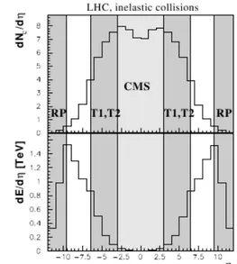
The TOTEM apparatus was designed to accomplish the TOTal cross section, Elastic scattering and diffractive dissociation Measurement, and thanks to its coverage for charged particles at high η, it represents the ideal tool for studying forward phe-nomena. About the 99.5% of all non diffractive minimum bias events and 84% of all diffractive events are triggerable by the inelastic telescope (T1,T2). This is of great importance to perform the total cross-section measurement with the luminosity-independent method, based on the Optical Theorem. Figure 2.1 shows the TOTEM detectors η_{− φ coverage, where the good coverage at high pseudo-rapidity values} can be appreciated. Furthermore figure 2.2 shows the expected particle multiplicity and energy flow as a function of η and it is clearly visible how the TOTEM detectors cover a region with high particle multiplicity and energy flow.

2.1 The total proton-proton Cross-Section

The total p-p cross-section (σtot) reflects the various interactions between the

col-liding particles and their constituents. Therefore a precise measurement of this quantity allows to distinguish between several existing theoretical models of soft proton interactions. The aim is to achieve a precision of about 1÷2 mb correspond-ing to_{∼1% of the expected total cross-section at the LHC energy of} √s = 14 TeV. Indeed, referring to figure 2.3 in which various existing measurements of σtot are

shown, a cross-section typically from 90 to 130 mb is expected, depending on the 25

(28)

26 2.1 The total proton-proton Cross-Section

Figure 2.1: Coverage in the pseudorapidity (η) and azimuthal angle (φ) of different de-tectors.

Figure 2.2: Charged particle multiplicity and energy flow as a function of the pseu-dorapidity for inelastic events (at √s = 14 TeV).

model used for the extrapolation. As mentioned above, the luminosity-independent method used by TOTEM for its measurement of the total cross-section relies on the Optical Theorem, written in equation 2.1, where F(t=0) is the forward elas-tic scattering amplitude for a squared four-momentum transfer t = 0 and k is the momentum in the center of mass.

σtot =

4π

k Im{F (t = 0)} (2.1)

From this theorem it follows the equation 2.2 that relates σtot with the luminosity

L, the nuclear part of the elastic cross-section dNel

dt and the parameter ρ (see 2.3).

Lσtot2 = 16π 1 + ρ2 · dNel dt ! ! ! ! t=0 (2.2) ρ = Re[F (t = 0)] Im[F (t = 0)] (2.3)

(29)

2.1 The total proton-proton Cross-Section 27

Figure 2.3: Fits from the COMPETE collaboration [15] to all available p-p and p-p scattering data with statistical (blue solid) and total (green dashed) error bands.

(30)

28 2.1 The total proton-proton Cross-Section

The additional following relation, that involves the inelastic rate Nineland the elastic

one Nel, is also clearly valid:

Nel+ Ninel = L σtot (2.4)

Therefore, the previous 2.2 and 2.4 form a system of two equations which can be solved either for σtot or L and lead respectively to the equation 2.5 and 2.6.

L = 1 + ρ 2 16π · (Nel+ Ninel)2 dNel/dt|t=0 (2.5) σtot = 16π 1 + ρ2 dNel/dt|t=0 Nel+ Ninel (2.6) Hence the quantities to be measured are the following:

• Ninel which will be measured by the inelastic telescopes T1, T2 and consists of

diffractive (_{∼ 18 mb) and non diffractive minimum-bias (∼ 65 mb) events. For} this purpose T1 and T2 also provide the reconstruction of the primary vertex in order to discriminate between the beam-beam events and the background ones (mainly from beam-gas interactions and muons halo).

• Nel which will be measured by the Roman Pots.

• dNel

dt

! !

t=0 which will be measured down to −t = 10−3 GeV

2 _{and then}

extrapo-lated to t=0.

For this measurement it is important that all TOTEM detectors have trigger capa-bility. Moreover particular beam optics conditions are required. In fact the proton detection by the Roman Pot (RP) stations at very small scattering angles (_{∼ few} µrad) requires special accelerator optics configurations. In particular a high β∗ function is needed, because the detection of protons elastically scattered so close to the beam axis requires a small beam angular divergence at the interaction point σθ ∼

"

1

β∗ (small with respect to the scattering angle itself). In addition, the

pro-ton revealed in the RP is required to be reasonably away from the beam envelope (σenv), typically at least 10 σenv. To perform the total cross section measurement

(31)

2.2 The elastic cross-section measurement 29

with the required precision of 1 _{÷ 2 % an optical configuration with β}∗ _{= 1540 m}

is desirable, for which a parallel-to-point-focusing condition is reached for the RP placed at 220 m from IP. This condition is important in order to eliminate the de-pendence on the transverse position of the proton at the collision point, allowing a more precise measure of the scattering angle. Even if a very high β∗ _{(1540 m) run}

is not foreseen for the early stage of LHC, there will be probably soon a run at an intermediate β∗ _{= 90 m. This will allow TOTEM to make a measurement of the}

total cross section with a∼ 5% uncertainty. For this β∗ _{= 90 m run the systematic}

error for the measurement will be dominated by the extrapolation of the nuclear elastic cross section to t = 0 (∼ 4% for -t measured down to -t ∼ 10−2 _GeV2 _),

while for the measurement at β∗ _{= 1540 m the total inelastic rate will give the main}

systematic uncertainty. In particular the uncertainty will be determined mainly by trigger losses in Single Diffractive events (_{∼ 0.8%). This occurs when the invariant} mass of the fragmented system is quite low (below 10 GeV/c2 _{) so that the particle}

pseudo-rapidities is beyond the T2 tracker acceptance [16]. Finally the theoretical uncertainty related to the estimate of the ρ parameter is expected to give a relative uncertainty contribution of less than 1.2% [15].

2.2 The elastic cross-section measurement

In order to distinguish among different models of soft proton interactions, the study of large impact parameter collisions such as elastic scattering processes is of great interest. High energy elastic nucleon scattering is a process for which many precise experimental data, covering a large energy range, are available. The predictions for the differential cross section of elastic proton-proton scattering, for an energy of √

s = 14 TeV, according to several different models [17], are shown in figure 2.4. Depending on the physics of the interaction involved, we can then distinguish several regions in squared transverse momentum t:

• |t| < 10−5 _GeV2_{: The elastic scattering is dominated by the exchange of one}

photon; it is called Coulomb region and it follows the Rutherford formula

dσ

dt ∼

1 t2.

(32)

30 2.2 The elastic cross-section measurement

Figure 2.4: Prediction from some different theoretical models for differential cross-section of elastic scattering. Also the acceptance ranges in |t| for different beam optics are shown.

• 10−3 _GeV2 _< _{|t| < 0.4 GeV}2_{: This is called the hadronic region and its}

theoretical description relies on the single pomeron exchange model. The dif-ferential cross section behaviour is roughly exponential dσ_dt ∼ e−B|t| _{but the}

slope is t dependent B(t) = d

dtln

dσ

dt. This shows a small model dependent

deviation from the exponential behaviour and it leads to a theoretical uncer-tainty that contributes to the systematic error of the total cross-section mea-surement. This region is important (together with the “interference” region 10−5 _GeV2 _<

|t| < 10−3 _GeV2_{) to evaluate the} dNel

dt

! !

t=0.

• |t| > 0.4 GeV2: This is the region in which the diffractive structure of the proton is visible. In fact we can see (from figure 2.4) the shape with maxima and minima that is typical of diffraction.

• |t| > 1.5 ÷3 GeV2_{: The predicted behaviour for the cross section in this region}

is proportional to _|t|−8_{, it relies on the description of central elastic collisions}

by perturbative QCD for example in terms of three gluon exchange [18]. This region is also useful to test the validity of different models because of the big

(33)

2.3 The diffractive process 31

difference in their predictions in this range.

With different running conditions and optics the TOTEM experiment will cover a wide t-range, measuring the elastic scattering from 2×10−3 _GeV2_{to about 10 GeV}2_.

This is really important to discriminate among different models (figure 2.4) for the differential cross-section of elastic scattering.

2.3 The diffractive process

The diffractive process comprises Single Diffraction (SD), Double Diffraction (DD), “Double Pomeron Exchange” (DPE, or Central Diffraction) and high order pro-cesses (“Multi Pomeron Exchanges”). These propro-cesses are expected to give a great contribution (about 50 mb together with the elastic scattering) to the total cross section at LHC. All these processes are characterized by a well defined topology in the pseudorapidity-azimuth (η− φ) plane, shown in figure 2.5, that allows to distin-guish between the various kind of diffractive events or non diffractive Minimum Bias (MB) events. The diffractive processes can be divided into “soft” and “hard”. The former gives almost the overall contribution to the diffractive cross-section, while the latter can be distinguished for the presence of jets in most of their final states. Moreover the main features of these processes are a large, non-exponentially sup-pressed, rapidity gap and no exchange of quantum numbers between the colliding protons. A large rapidity gap, usually greater than 2 pseudorapidity units while non-exponentially suppressed, means that the probability of finding the gap in the final state is not a strong function of the gap width. An example for these events can be provided by SD processes at HERA (e + p→ e + p + X), where X represents the fragmented system and has an invariant mass Mx. In the approximation of s, Mx '

1GeV2 the rapidity gap ∆η is related to Mx via the relation ∆η =− ln

#M2 x

s $

. Since it is supposed that quantum numbers are not exchanged between the colliding pro-tons, this leads to study diffractive processes in terms of Pomeron exchange. In hard diffractive processes the Pomeron is identified as a colorless gluon ladder exchanged by partons. However, there is not yet a satisfying theory which can explain all the aspects of this kind of hadronic processes and the understanding of the nature of

(34)

32 2.3 The diffractive process

Figure 2.5: Typical event topology in the η − φ plane for non diffractive (Minimum

Bias) and diffractive processes (SD, DD, DPE, Multi Pomeron processes). The relative cross section values, measured at Tevatron and expected at the LHC respectively, are also reported on the right column.

(35)

2.3 The diffractive process 33

Pomeron interactions is still a big challenge. Another important feature of diffractive events is that the majority of them show “leading” protons in the final states. These leading protons appear intact from the interaction region and are characterized by their t and by their fractional momentum loss ξ≡ ∆pp ∼

Mx

s . According to the beam

optics, these leading protons can be revealed with high efficiency by the TOTEM RP detectors. Even if TOTEM is able to measure ξ, t, and mass-distributions in soft DPE and SD events, in order to have the possibility to perform detailed studies of the full structure of diffractive events (with the optimal reconstruction of one or more sizeable rapidity gaps) the integration of TOTEM with the CMS detectors would be welcome. For this purpose the TOTEM triggers are designed to be also incorporated into the general CMS trigger scheme and common data taking [19] are foreseen in a later stage.

(36)

(37)

Chapter 3 Tuning of Geant4 simulation

Nowadays in high energy physics an important role is played by simulation. In fact, due to the increasing complexity of the experiments, simulating the detectors response is a fundamental tool in order to understand the physical processes under investigation. The simulation is especially useful to determine detection biases, measurement errors, background contribution and to estimate quantities which can be difficult to determine with a direct measurement. For these reasons it is important to have an optimal tuning of the simulation. In this chapter, after a brief introduction to the Geant4 simulation package, the work done, in order to have a better tuning of the simulation of interest for any analysis involving the T2 detector, is reported.

3.1 A brief introduction to Geant4

TOTEM is using the same software framework of CMS (CMSSW). CMSSW provides in particular an interface for various software tools like ROOT, Geant4, several MC generators (Pythia, Phojet, and so on..), the Iguana visualisation software and many others. In particular, Geant4 (acronym of GEometry ANd Tracking) [13] is a platform for the simulation of the passage of particles through matter using Monte Carlo methods. It’s based on object oriented programming (C++ language) and it is a software toolkit developed at CERN. At the heart of Geant4 there is an abundant set of physics models which handle the interactions of particles with matter across a very wide energy range, allowing to reproduce the detector geometry and response,

(38)

36 3.1 A brief introduction to Geant4

Figure 3.1: Main components of the CMS detector.

as well as the decay processes of secondaries. The physical layout of an experiment (including detectors and passive materials) can be so schematized in the Geant4 geometry files and it is used by the simulation software to “evolve” a given physics event from the MC generation level (“particle level”) to the signals observed in the detectors (“digitization”).

In the CMSSW framework the Geant4 geometry is reproduced via the xml based Detector Description Language (DDL) [20]. The idea behind this detector descrip-tion is that the informadescrip-tion about the detector can be represented with a tree in which the nodes represent certain detector parts, and the edges represent a “part of” relationship. Every node in the tree can be uniquely mapped to a part or to a collec-tion of parts in the “real” detector. The detector descripcollec-tion in CMSSW consists of a hierarchy of geometry descriptions, based on direct acyclic multi graphs (acyclic multi graphs can be unfolded into a tree). Furthermore, this hierarchy contains parameters that give a detailed description about elements within this geometry de-scription. To prevent a “part explosion”, i.e. the replication for several times of the descriptions of identical parts of the detector, the graph contains two layers of

(39)

de-3.2 Geant4 cuts tuning 37

scriptions. A “part-type” containing the material and solid shape information, and a collection of parts position. A part of the detector is described by a “part-type” and its position relatively to another part-type (called parent part-type). Furthermore, a part can have a “parameterised” position. This is a description of a part that permits to place it several times in a parent part-type. In the xml files a number denotes a parameterisation of the parts. Attached to every part-type will be in-formation about its material and geometry. Moreover certain parts (or part-types) have specific parameters related to their particular role (for example a silicon sensor can have a parameter “number of strips”).

3.2 Geant4 cuts tuning

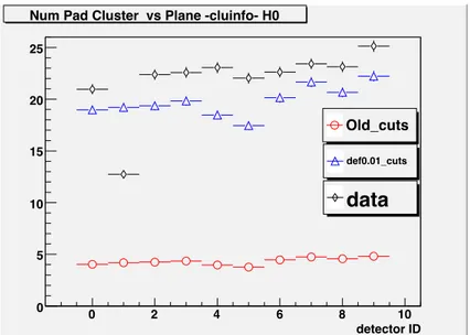
Due to the big mismatch between data (collected with the T2 inclusive inelastic trig-ger in low luminosity runs, where the pile-up probability is negligible) and simulation (inelastic processes from Pythia MC [10]) observed in a first study of the T2 detector occupancy (as shown in figure 3.2), it was clear the importance to check the good-ness of the simulation of the volumes in the forward region, which could affect the T2 telescope response. A comprehensive study has then been performed in order to check the proper Geant4 implementation and tuning of the simulation of the Beam Pipe, of the CMS components of interest and of the T2 detector. While dealing with the T2 geometry simulation optimization in the next section, in the present one we focus our attention on two fundamental aspects of the CMS simulation tuning: the cut parameters and the list of included volumes. To have an idea of the most im-portant volumes to simulate properly for the T2 detector in figure 3.1 the CMS [21] experimental apparatus with its subdetectors is shown. The cut parameters define ranges in the different materials, so that particles with a range lower than the cut parameters value are not generated in the simulation (which anyway properly takes into account their energy deposition). The cuts used in the simulation are basically of two types: the so called “default cut” and the “cuts per region”. The default cut affects all the simulated volumes; the cuts per region affect only some “selected” volumes (listed in appropriate files). All the volumes, representing the CMS and

(40)

38 3.2 Geant4 cuts tuning detector ID 0 2 4 6 8 10 0 5 10 15 20 25 Old_cuts def0.01_cuts data

Num Pad Cluster vs Plane -cluinfo- H0

Figure 3.2: Average number of pad clusters in each plane of the H0 T2 quarter (detector

Id from 0 to 9). Comparison between data (black diamonds), simulation with improved default cut without cuts per region (blue triangles) and the old default cut (red circles). The low occupancy of plane 1 observed in data is due to an electric short on it, whose effect is not included in the simulation.

TOTEM detectors, that will be simulated by Geant4 are specified in a “global” list. The optimization of these cuts is clearly very useful in order to save CPU time. On the other hand, the CMS volumes (detector components) can be included or not in the simulation (acting on the global list), depending on their impact on the T2 detector response. While it is necessary to check if all of the volumes of interest are included in the simulation, the optimization of this list is also important in order to save CPU time (by removing the ones not affecting T2).

To perform this study the attention is focused on some interesting observables to check if a change in cuts or volumes would have some effect on the T2 detector response. We decided to consider the average pad cluster multiplicity per each plane, being the T2 detectors more efficient and less subject to noise in the more granular pad channel readout. Moreover this observable is simple (and so less biased, e.g. by tracking or alignment effects) and is directly related to detector occupancy, hence to the simulation response. Only the results related to the H0 (“plus near”: west, internal ring location) T2 quarter are report here; similar results have been obtained when considering the other three quarters. A proper tuning of the model reproducing the digital response of the detector, in terms of strip and pad cluster

(41)

3.2 Geant4 cuts tuning 39

efficiency and size distribution (“Digitization”), has already been performed using test-beam and Ion Collision data [22]. The goal is to find a “stable” configuration that uses the minimum CPU time, i.e. to reach a condition in which adding more volumes or pushing the cuts to a lower value does not have any substantial effect on the detector response. To achieve this result a lot of comparison between different simulation are shown in various plot. To ensure the best possible comparison all the simulation in a same plot are made with the same generation seeds, in order to avoid discrepancies due to difference in the physical events simulated. Anyway could happen that some events crash in a simulation and not in another. When is possible we correct on this crashed events, removing manually the corresponding ones from the simulation that don’t have the crashes, but is not always completely possible, so some little difference in the number of events between the two simulation could occur.

3.2.1 Geant parameters tuning

The simulation considered until now was using the default cut set to 1000 mm, defining the sampling range in the material, and the cuts per region set to values depending on the “selected” volumes of interest: all TOTEM detectors plus the beampipe from z = 0 m up to z = 6.5 m (set to 1 mm); the forward shielding around the T2 telescope (sampling set to 10000 mm). The results obtained with this simulation, which we will call ‘old default’ selection, are shown in figure 3.2, where they are compared with the data and with a simulation performed by setting the default cut to 0.01 mm without applying any cut per region. It seems clear that there is a huge difference between data (black diamonds) and simulation (red circles) that we can considerably reduce by moving the cut in the whole CMS volume to a lower value (blue triangles). However, as expected, this setting increases greatly the CPU time used in the simulation. So, for an optimal tuning also in terms of timing, it is important to understand what are the regions of importance for T2, so to reduce the cut value only there. A first check in this direction is reported in figure 3.3, where the red circles represent the results with the “old default cut” while the blue triangles represent the same situation in which we change only the value

(42)

40 3.2 Geant4 cuts tuning detector ID 0 2 4 6 8 10 0 5 10 15 20 25 Old_cuts OldCutRegion_weakerCut data

Figure 3.3: Comparison between data (black diamonds), default sampling cut set to 1000

mm with cuts per region set to 0.01 (blue triangles) and the “Old cuts” (red circles). The low occupancy of plane 1 observed in data is due to an electric short on it, whose effect is not included in the simulation.

of the cuts per region parameter, setting it to 0.01 mm. We can see a little increase in the average pad cluster multiplicity, but the difference between simulation and data (black diamonds) is still huge. This means that there are some volumes not yet

detector ID 0 2 4 6 8 10 0 5 10 15 20 25 NewCutRegion_0.01 OldCutRegion_0.01 data

Figure 3.4: Comparison between data (black diamonds) and default cut set to 1000 mm

with cuts per region set to 0.01 mm, with two different volumes choices for the cuts region (red and blue markers). The cuts region represented by the red circles includes also the beampipe from 6.5 to 16 m, the beam radiation monitors and Castor. The low occupancy of plane 1 observed in data is due to an electric short on it, whose effect is not included in the simulation.

(43)

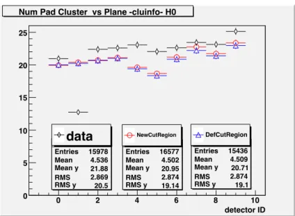
considered in the “selected” region which are really important for our detector. So we started to add additional volumes of potential interest, by including in the cuts region list the missing section of the beampipe (from 6.5 m up to 16 m), the beam radiation monitors and the Castor calorimeter. The result of this improvement is shown in figure 3.4 (red circles), where it is also compared with the data (black diamonds) and the previous situation in which no additional volume was included in the cuts per region list (blue triangles). We can see that this addition of volumes has a significant effect on the simulation and that now the result of using low cuts (0.01 mm) only for the volumes of interest is quite similar to the one obtained by applying low cuts to the whole CMS detector (setting the default cut to 0.01 mm). This is shown in figure 3.5, where the result obtained with only the default cut set to 0.01 mm (blue triangles) is directly compared with the one obtained with default cut set to 1000 mm and cuts per region set to 0.01 mm for the “improved” selected volume list (red circles).

NumPadCluVsPlaneAll3H0 Entries 16577 Mean 4.502 Mean y 20.95 RMS 2.874 RMS y 19.14 detector ID 0 2 4 6 8 10 0 5 10 15 20 25 NumPadCluVsPlaneAll3H0 Entries 16577 Mean 4.502 Mean y 20.95 RMS 2.874 RMS y 19.14 NewCutRegion NumPadCluVsPlaneAll3H0 Entries 15436 Mean 4.509 Mean y 20.71 RMS 2.874 RMS y 19.1 NumPadCluVsPlaneAll3H0 Entries 15436 Mean 4.509 Mean y 20.71 RMS 2.874 RMS y 19.1 DefCutRegion NumPadCluVsPlaneAll3H0 Entries 15978 Mean 4.536 Mean y 21.88 RMS 2.869 RMS y 20.5 NumPadCluVsPlaneAll3H0 Entries 15978 Mean 4.536 Mean y 21.88 RMS 2.869 RMS y 20.5 data

Figure 3.5: Comparison between data (black diamonds), simulation with default cut set

to 0.01 mm (blue triangles) and simulation with default cut set to 1000 mm and cuts per region set to 0.01 mm on the “improved” list (red circles). The low occupancy of plane 1 observed in data is due to a electric short on it, whose effect is not included in the simulation.

(44)

42 3.2 Geant4 cuts tuning

3.2.2 Getting the correct list of selected volumes

From figure 3.5 we can see that there is a residual mismatch between data and simulation, indicating there is still some important volume not included in the proper lists. After a first check, we found for instance that the HF calorimeter (CMS Hadron Forward calorimeter) is not included at all in the simulation, i.e. in the global volumes list that defines the simulated geometry of CMS. We then included HF, both in the global volumes list and in the cuts per region list and redo the simulation. The results are shown in figure 3.6, where the red circles represent the previous situation, the black diamonds are related to only the default cut set to 0.01 mm with HF included in the geometry and the blue triangles describe the inclusion of HF in the cuts per region list (and obviously in the geometry too). With HF included we have a decrease in the average pad cluster multiplicity, evidently as a consequence of some shielding effect on T2, and an increase in the difference between data and simulation.

NumPadCluVsPlaneAll3H0 Entries 16132 Mean 4.501 Mean y 20.96 RMS 2.875 RMS y 19.15 detector ID 0 2 4 6 8 10 0 5 10 15 20 25 NumPadCluVsPlaneAll3H0 Entries 16132 Mean 4.501 Mean y 20.96 RMS 2.875 RMS y 19.15 GoodCut NumPadCluVsPlaneAll3H0 Entries 16403 Mean 4.5 Mean y 17.52 RMS 2.879 RMS y 18.68 NumPadCluVsPlaneAll3H0 Entries 16403 Mean 4.5 Mean y 17.52 RMS 2.879 RMS y 18.68 GoodCut+HF NumPadCluVsPlaneAll3H0 Entries 16451 Mean 4.506 Mean y 17.33 RMS 2.878 RMS y 18.78 NumPadCluVsPlaneAll3H0 Entries 16451 Mean 4.506 Mean y 17.33 RMS 2.878 RMS y 18.78 deffCut0.01CutRegOFF+HF Num Pad Cluster vs Plane -cluinfo- H0

Figure 3.6: Comparison between the default cut set to 1000 mm with cuts per region

set to 0.01 mm without HF (red circles) and with HF included (blue triangles). The black diamonds show a simulation with only default cut set to 0.01 mm and HF included.

From this example it is clear that it is important to properly check if all the CMS volumes potentially of interest are included in the simulation. As first step the default cut is set to 0.01 mm (no cuts per region) for *ALL* the CMS volumes and the obtained result is used as “benchmark” to properly tune the volume list

(45)

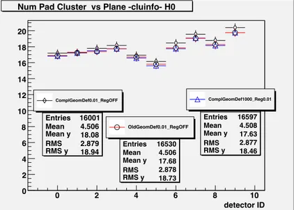
and parameter value for the cuts per region option. As usual, the reason for this additional tuning is the minimization of the CPU time required for the simulation. Following this perspective we then added to the global volume list other volumes still not included: CMS tracker, calorimeters and muon detectors. The results are shown in figure 3.7, where the black diamonds represent the “benchmark” situation and the blue triangles the one with the new global geometry, the default cut set to 1000 mm and the cuts per region set to 0.01 mm (with the selected volume list unchanged). The red circles instead represent the situation with the old geometry, the default cut to 0.01 mm and no cuts per region. The comparison between black diamonds

NumPadCluVsPlaneAll3H0 Entries 16597 Mean 4.508 Mean y 17.63 RMS 2.877 RMS y 18.46 detector ID 0 2 4 6 8 10 0 2 4 6 8 10 12 14 16 18 20 NumPadCluVsPlaneAll3H0 Entries 16597 Mean 4.508 Mean y 17.63 RMS 2.877 RMS y 18.46 ComplGeomDef1000_Reg0.01 NumPadCluVsPlaneAll3H0 Entries 16001 Mean 4.506 Mean y 18.08 RMS 2.879 RMS y 18.94 NumPadCluVsPlaneAll3H0 Entries 16001 Mean 4.506 Mean y 18.08 RMS 2.879 RMS y 18.94 ComplGeomDef0.01_RegOFF NumPadCluVsPlaneAll3H0 Entries 16530 Mean 4.506 Mean y 17.68 RMS 2.878 RMS y 18.73 NumPadCluVsPlaneAll3H0 Entries 16530 Mean 4.506 Mean y 17.68 RMS 2.878 RMS y 18.73 OldGeomDef0.01_RegOFF

Figure 3.7: Simulation with only the default cut set to 0.01 mm with all the CMS volumes

included (black diamonds) compared to a simulation on the same geometry and default cut set to 1000 mm, cuts per region set to 0.01 mm (red circles). And with a simulation (blue triangles) with default cut to 0.01 (no cut per region) and the old geometry (no CMS tracker, calorimeters and muon detectors).

and red circles markers shows that some volumes in the previous simulation were missing, while the comparison between black diamonds and blue triangles markers indicates that in the new simulation some volumes are missing in the cuts per region list.

We then included in the cuts per region list also the CMS central region (tracker, calorimeters, muon detectors). Because of software problems (a big amount of crashes) arising when applying weak cuts (like 0.01 mm) in the whole volume of these additional CMS detectors, we used for them some cut lists already defined

(46)

in-44 3.2 Geant4 cuts tuning

side the CMS software framework. These lists have different cuts value for different part of the detectors, but on average the value is about 1 mm. The plot of figure 3.8 shows the comparison between the usual benchmark simulation represented in black diamonds and the new one depicted in blue triangles. From this plot it can argue that there is some volume in the central region of CMS that gives some contribu-tion to the pad cluster multiplicity in T2. In fact now there is no more difference between the benchmark simulation and the new one with the use of cuts per region, meaning that now it is included some important volume that was excluded in the previous simulation. It was found that the origin of this contribution is the CMS Hadronic calorimeter “Hcal”, as shown in figure 3.9. Here the benchmark simulation (black diamonds) gives similar results with respect to another simulation obtained by adding only Hcal to the usual selected volume list (beampipe, forward shielding, Castor and TOTEM detectors) to which the cuts per region are applied. It is very

NumPadCluVsPlaneAll3H0 Entries 15157 Mean 4.507 Mean y 18.01 RMS 2.879 RMS y 19 detector ID 0 2 4 6 8 10 0 2 4 6 8 10 12 14 16 18 20 NumPadCluVsPlaneAll3H0 Entries 15157 Mean 4.507 Mean y 18.01 RMS 2.879 RMS y 19 CmplVol_Def0.01 NumPadCluVsPlaneAll3H0 Entries 15666 Mean 4.511 Mean y 18.07 RMS 2.876 RMS y 18.94 NumPadCluVsPlaneAll3H0 Entries 15666 Mean 4.511 Mean y 18.07 RMS 2.876 RMS y 18.94 NumPadCluVsPlaneAll3H0 Entries 15666 Mean 4.511 Mean y 18.07 RMS 2.876 RMS y 18.94 CmplVol_Def1000_Reg0.01+AllCMScut

Figure 3.8: Comparison between the simulation with only default cut set to 0.01 mm

on all CMS volumes (black diamonds) and the one (blue triangles) with default cut set to 1000 mm and cuts per region in the usual volumes (beampipe, HF, forward shielding, Castor and TOTEM detectors) set to 0.01 mm, and in addition to tracker, calorimeters and muon system (average cut value set to 1 mm).

important to notice that this choice of cuts, besides getting the same results, allows us to reduce the CPU time of about 30% with respect to the benchmark simulation in which we use only low default cuts on all CMS volumes. In order to further reduce the CPU time, we tried to remove other volumes (potentially not contributing to