UNIVERSITÀ DEGLI STUDI DI ROMA
"TOR VERGATA"
FACOLTA' DI ECONOMIA
DOTTORATO DI RICERCA IN
ECONOMIA DELLE ISTITUZIONI E DEI MERCATI MONETARI E
FINANZIARI
XX CICLO
Empirical Essays on Corporate Finance
and Government Bond Markets
Chiara Coluzzi
Docente Guida/Tutor: Prof. Michele Bagella
Coordinatore: Prof. Gustavo Piga
Contents
Chapter 1: Do financing obstacles hamper firm growth? Evidence on euro area non financial corporations.
Chapter 2: The pricing of the option implicitly granted by the Italian Treasury to the Specialists in the reserved auction reopening.
Chapter 3: Measuring and Analyzing the Liquidity of the Italian Treasury Security Wholesale Secondary Market (with Sergio Ginebri and Manuel Turco).
C
HAPTER
1
DO FINANCING OBSTACLES HAMPER FIRM GROWTH? EVIDENCE ON
EURO AREA NON FINANCIAL CORPORATIONS∗
Abstract
This paper investigates whether financial factors, along with firms’ characteristics, significantly affect firm growth using an unbalanced panel of about 1,000,000 observations for around 155,000 non-financial corporations in five Euro area countries. In addition to the balance sheet information in the panel, I also rely on firm-level survey data. In this way it is possible to work out a direct measure of the firms’ probability of facing financing obstacles. Furthermore, I find that firm growth is not due to chance and that financial position matter. Although the evidence that firm cash flow and growth opportunities positively affect growth is unambiguous, I obtain less clear-cut results for leverage and debt burden ratios. Moreover, even if the direct measure of financing obstacles is a function of qualitative indicators, it is able to capture the negative impact of financing obstacles on firm growth in four countries.
Keywords: Financing Constraints, Firm Growth, Panel Data. JEL Classification: C23, E22, G32, L11.
∗ Acknowledgments: This paper draws from a project on firm growth conducted while I was a trainee at the European Central Bank (ECB), Capital Market and Financial Structure Division. I am particularly indebted to A. Ferrando and C. Martìnez-Carrascal for their supervision and support during and after that period. I also wish to thank F. Drudi, P. Hartmann, S. Scarpetta and other participants in the ECB Workshop on Finance, Growth and Productivity, and in the internal seminar in the Capital Markets and Financial Structure Division. I am grateful to G. Piga, G. Spagnolo, R.J. Waldmann and other participants in the Tor Vergata Workshop for Doctorate Students in Money and Finance, in the SUERF Conference, Paris, in the DIME Workshop, Pisa. Finally, I thank an anonymous referee for useful comments. The views expressed are those of the author and should not be attributed to the ECB. Correspondence address:
1. Introduction
Studying firm growth can provide insights into the dynamics of the competitive process, strategic behaviour, the evolution of market structure, and, perhaps, even the growth of the aggregate economy (Carpenter and Petersen, 2002). However, there are just a few studies that examine the finance-growth nexus at the firm level. As surveyed by Wachtel (2003), Levine (2005) and Papaioannou (2007), usually they assess the effect of well-developed financial markets in relaxing firm’s financing constraints and do not address directly the role of financing constraints on growth. Even when financing constraints are investigated, the focus is on firms’ investment choices and it is only indirectly proved that they affect investment decisions and then firms growth (Hubbard, 1998).
This study aims at providing a useful contribution to the understanding of the main factors affecting firm growth, and insights on the importance of enhancing firms’ funding opportunities. Its main contribution is the direct measurement of the impact of firms’ financial position and access to finance on growth. In doing this, it also adds to the literature on both stochastic and deterministic approaches to explain the determinants of firm size. With respect to the former, I refer to the Law of Proportionate Effects (LPE) (Gibrat, 1931), that states that firm growth is independent of initial size and past growth rates. Both Sutton (1997) and Hart (2000) survey the empirical tests of LPE and the earlier literature trying to explain the departure from this law. This departure was also explained in terms of financing constraints (Cooley and Quadrini, 2001; Cabral and Mata, 2003; Albuquerque and Hopenhayn, 2004; Clementi and Hopenhayn, 2006). Asymmetric information and financing constraints are also considered in the deterministic approach, as reviewed by Schiantarelli (1996), Hubbard (1998) and Stein (2003). Through the estimation of an augmented version of the standard LPE equation I jointly test the implications of both strands of literature.
The novelty of this research is to make use of the survey data advantages to overcome balance sheet data shortcomings and vice versa. On the one hand, surveys might be affected by self-reporting bias, but, on the other hand, they provide qualitative and direct information on the firms’ situation that cannot be derived from balance sheet data. The latter offer relevant information on the firms’ financial position itself, although both cash flow (as in Fazzari, Hubbard and Petersen, 1988) and other balance sheet based indexes (as in Kaplan and Zingales, 1997b, and Whited and Wu, 2006) may either be a bad proxy for the access to the loan market or capture effects not related to liquidity constraints. Hence, I construct a direct indicator of financing obstacles reported by firms from firm-level survey data (WBES by the World Bank, 2000), which can be used to exploit the richness of information of a larger panel dataset.
As in Carpenter and Petersen (2002), I investigate the impact of cash flow on firm growth. Furthermore, referring to Bernanke, Gertler and Gilchrist (1996), Lang, Ofek and Stulz (1996) and Nickell and Nicolitsas (1999), I contribute to the literature on financial distress and firm performance by including variables such as the indebtedness level or the debt burden that can affect the external finance premium faced by firms. With respect to the econometric methods, I apply dynamic panel data techniques as in Oliveira and Fortunato (2006b) and Hutchinson and Xavier (2006).
Another major difference with earlier literature is that my dataset includes mainly non-listed and small and medium-sized firms. In particular, I use a panel dataset of around 1 million firm-year observations, 95% of them being SMEs, in five euro area non-financial corporations (namely France, Germany, Italy, Portugal and Spain). This is a clear advantage with respect to most previous studies, since these are the firms expected to be more affected by financing constraints, and are the backbone of the EU’s non-financial business economy.1
After controlling for growth opportunities, as well as time and sectoral effects, I analyze the impact on growth of firm size, age, financial position and probability of encountering financing obstacles. I find that my indicator of financing obstacles has a significantly negative effect on firm growth and that financial position matters. In effect, while evidence of the positive role of cash flow on firm growth is unambiguous, results on leverage and debt burden are less clear-cut. In addition, LPE is clearly rejected in three out of the five countries under analysis.
The rest of the paper is organized as follows: after reviewing the existing literature in section 2, I present the datasets and summary statistics in section 3. Section 4 states the steps of the analysis and the empirical model, while in section 5 I discuss the estimation results. Section 6 concludes.
2. Review of Literature
As reviewed by Hart (2001), there is a vast literature on the theories of firm growth. In particular, we can distinguish between a stochastic and a deterministic approach to explain the determinants of firm size. The former argues that in a world with no differences ex ante in profits, size and market power across firms, all changes in size are due to chance. The latter assumes, on the contrary, that growth rate of firms differs because of observable industry and firm specific characteristics.
This paper draws from both approaches to investigate the relationship between financing obstacles and firm growth. With respect to the stochastic approach, I relate to the so called Law of
Proportionate Effects. Put forward by Gibrat in 19312, LPE states that factors that influence firm growth, such as growth of demand, innovation, etc., are distributed across firms in a manner which cannot be predicted from information about firm’s current size or its previous growth performance. In the past decades, LPE has been extensively tested for many different countries with mixed empirical results.3 In effect, it comes out that LPE may hold in particular points in time, for some sectors and/or size classes, but evidence of faster growth of smaller firms suggests that size is often linked to some systematic factors.4 Age also seems to play a role, for instance because it implies learning (Jovanovich, 1982). Evans (1987a and 1987b) and Dunne, Roberts and Samuelson (1988 and 1989) investigate both size and age effects on growth and find two statistical regularities in their analyses. First, firms’ probability of surviving is increasing in size, but, conditional on survival, small firms grow faster.5 Second, given size, young firms grow faster, but they have a smaller probability of survival.
LPE test is also complicated by two econometric issues. The first concerns the heteroskedasticity arising if the Law is not confirmed, i.e. if small firms grow faster than their larger counterparts, the variance of growth should tend to decrease with size. The second issue was put forward by Chesher (1979) and relates to the inconsistency of ordinary least squares estimators if growth is serially correlated. In the present paper both issues are controlled for.
More recently, a number of theoretical papers explain the departure from the LPE in terms of financing constraints. Cooley and Quadrini (2001) show how a combination of persistent shocks and financial frictions can account for the simultaneous dependence of firm dynamics on size and age. Cabral and Mata (2003) explain the empirical right-skewed firm size distribution with the fact that firms cease to be financially constrained. The authors develop a two period-model of a competitive industry. In the first period the firm may be financially constrained, thus size is the minimum between the optimal size and the size affordable by the entrepreneur; in the second, when the firm is no longer affected by financing constraints, size is at its optimal level. In addition, both Albuquerque and Hopenhayn (2004), who study lending and firm dynamics in a model with limited enforcement, and Clementi and Hopenhayn (2006), who model the relationship between borrower
2 Gibrat observed that the size of firms followed the lognormal distribution very closely, from which he concluded that the firms’ rate of growth ought to be a random process.
3 Sutton (1997) provides a review of the theoretical and empirical literature. Among others, see also Mansfield (1962), Hall (1987), Evans (1987a, 1987b) and Goddard, McKillop and Wilson (2002) for USA, Hart and Oulton (1996), Kumar (1985) and Dunne and Hughes (1994) for UK, Goddard, Wilson and Blandon (2002) for Japan, Mata (1994) and Oliveira and Fortunato (2006a) for Portugal, Wagner (1992) and Harhoff, Stahl, Woywode (1998) for Germany, Solinas (1995) and Lotti, Santarelli and Vivarelli (2003) for Italy. Tschoegl (1983), instead, performs a multi-national study. 4 For instance, government small business policies or the need to reach the minimum efficient scale might explain faster growth of smaller firms.
5 This result might be affected by a sample selection bias, i.e. as slow growing firms are more likely to exit, small fast growing firms may be over-represented. Lotti, Santarelli and Vivarelli (2003) offer a survey of papers addressing this
and lender in the asymmetric information framework, reach very similar conclusions for firm dynamics. In particular, their models are consistent with the empirical findings that as age and size increase, mean and variance of growth decrease, and firm survival increases.
From a purely deterministic point of view, the impact of financing constraints on the real activity of firms is a well known issue, as reviewed by Schiantarelli (1996), Hubbard (1998) and Stein (2003). The main idea is that imperfections in capital markets produce a wedge between the cost of internal and external finance. In particular, asymmetric information between lender and borrower is the main source of this wedge (Meyers and Majluf, 1984). Nevertheless, both theory and empirical evidence focus on the effect of financing constraints on firms’ investment decisions, while fewer papers concentrate directly on firm growth. Carpenter and Petersen (2002) address the issue using a panel of small manufacturing US enterprises. They find that the growth of most firms in their sample is constrained by internal finance. Wagenvoort (2003) replicates the model for Europe, adding to the empirical analysis the impact of leverage and firm size, and finds that growth-cash flow sensitivities are decreasing in firm size. Oliveira and Fortunato (2006b) provide evidence that, in Portugal, smaller and younger firms have higher growth-cash flow sensitivities. Applying the same method used here for Belgian and Slovenian firms, Hutchinson and Xavier (2006) find that young firms and firms with long-term debt are most constrained and that micro and SMEs can face great difficulties in accessing external sources of finance. Fagiolo and Luzzi (2006) show on Italian data that the stronger liquidity constraints, the more size negatively affects firm growth.
Overall, the body of this literature implies the need for an a priori classification6 between financially constrained and unconstrained firms in order to check if the sensitivity of investment/growth to cash flow is higher for constrained than for unconstrained firms.7 I depart from this debate by making use of survey data to obtain a direct measure of financing obstacles. In this respect, I follow the approach of Beck, Demirgüç-Kunt and Maksimovic (2005) and Beck, Demirgüç-Kunt, Laeven and Maksimovic (2006) that exploit the firm-level information contained in the World Business Environment Survey (WBES) to investigate the effect of financial, legal, and corruption problems on firms’ growth rates. Survey data are also used, for instance, by Becchetti and Trovato (2002). They test Gibrat’s Law on different waves of a survey on Italian manufacturing
6 The splitting criteria focus on firms characteristics that are related to information costs. For instance, small and young firms should face more binding financing obstacles due to the more severe information asymmetries their creditworthiness analysis involves (Devereux and Schiantarelli, 1990; Gilchrist and Himmelberg, 1995). Foreign owned firms and firms belonging to a group (keiretsu in Hoshi, Kashyap and Scharfstein, 1991) should suffer less from financing constraints, as they have alternative source of finance. An investment grade rating for corporate bonds also reduces financing constraints (Whited, 1992).
7 Although many researchers argue that the correlation is due to financing constraints (see the seminal paper by Fazzari, Hubbard and Petersen, 1988 and 2000), others say that cash flow is simply a proxy for investment opportunities
firms. They include in the regression a dummy variable which takes value one if the firm reports to be credit constrained. Their analysis rejects LPE and shows that the inclusion of variables measuring the availability of external finance (subsidies, leverage and financing constraints) significantly affects firm growth.
Additionally, I complement the survey data with information on firms’ financial position using balance sheet information. Indeed, it is possible to exploit the survey based measure of financing obstacles to investigate directly the relationship between financing constraints and growth, without the need of splitting the sample according to any arbitrary a priori classification.
This paper also complements the literature about financial distress and corporate performance. Among others, Opler and Titman (2004) find that firms with high leverage are more likely to experience performance losses in industry downturns than other firms. Similarly, Bernanke, Gertler and Gilchrist (1996) observe that high leverage reduces the firms’ ability to growth through a liquidity effect. In particular, the economy is characterized by a financial accelerator. This implies that during recessions borrowers facing high agency costs should receive a relatively lower share of credit, and hence account for a proportionally greater part of the decline in economic activity. By contrast, Lang, Ofek and Stulz (1996) recognize that the relationship between financial distress and firm growth and performance may be sometimes ambiguous. On the one hand, leverage does not reduce growth for firms known to have good investment opportunities; on the other hand, leverage is negatively related to growth for firms whose growth opportunities are either not recognized by capital markets or are not sufficiently valuable to overcome the effects of their debt overhang. In this study, I check the impact of leverage on firm growth, and the role of debt burden, which also measures the degree of financial pressure faced by firms.8
Finally, this paper is also linked to the finance-growth literature. A large amount of research provides evidence that financial development has a significantly positive effect on economic growth.9 The literature has recently been moving from purely cross-country based analysis to a more micro oriented approach, as a way to alleviate some of the limitation of the cross-country analysis, such as reverse causality and multi-collinearity. Seminal papers, in this respect, are Rajan and Zingales (1998) and Demirgüç-Kunt and Maksimovic (1998) based on industry and firm-level data respectively. These papers assume that a well-developed financial system removes or reduces the barriers to external financing for firms. The former argues that industries that are more dependent on external financing should do better in countries with better financial systems.
8 See Nickell and Nicolitsas (1999), Hernando and Martínez-Carrascal (2008) and Martínez-Carrascal and Ferrando (2008).
Similarly, the latter claims that the proportion of firms that grow rapidly enough to require external financing is related to the development of the financial sector. However, only recently the availability of large firm level panel dataset is permitting to investigate the issue of the relationship between firm growth and the availability of finance. I contribute to this line of research focusing on more homogeneous countries (such as countries in the euro area). Guiso, Jappelli, Padula and Pagano (2004) and Ferrando, Köhler-Ulbrich and Pál (2007) focus on eurozone countries and find some evidence supporting the hypothesis that the lack of financial development constrains more severely the growth of SMEs, which tend also to be more financially constrained than large firms. Aghion, Fally and Scarpetta (2007), using harmonized firm-level data on entry and post-entry growth in 16 countries, find that finance matters most for the entry of small firms, especially in sectors that are more dependent upon external finance, and that financial development improves post-entry growth of firms. Inklaar and Koetter (2008), instead, exploit firm-level information to measure the dependence of industries on external finance and the efficiency of financial intermediaries within the EU-25. They find that the relative efficiency of banks in providing financial services is an important dimension of financial development. The difference with respect to these studies is that I measure directly the probability of having financing obstacles.
3. Data and Summary Statistics
Data come from two sources, WBES and AMADEUS, which are respectively a firm-level survey about constraints to firm growth and performance and a panel dataset collecting balance sheet information. The aim of the paper is to exploit the survey data advantages to overcome the balance sheet data shortcomings and vice versa. Accordingly, I incorporate both data sources to analyze the impact of the financial position of firms on their growth.
3.1 Measuring financing obstacles using survey data (WBES)
My measure of financing obstacles is based on the information derived from the World Business Environment Survey (WBES), which was carried out by the World Bank Group between 1999-2000 to identify obstacles to firm performance and growth around the world. In the questionnaire, the respondents are required to base their answers on the “perception and experience of doing business” in their country.10 Financial figures, instead, are based on estimation by the respondent over the previous one or three years. The time horizon is specified in the paper each time a new variable is introduced. Qualitative variables other than obstacles to growth, like size, refer to the time the questionnaire was administrated.
A fundamental property of WBES is that data are at the firm-level. In particular, WBES database is size-stratified and has excellent coverage of small and medium-sized firms, where small firms are those with 5–50 employees. Medium-sized firms are those that employ 51–500 employees, and large firms are those with more than 500 employees.11 Sectors are defined at a broad level and they include manufacturing, services, agriculture and construction. The survey was administered in such a way that the sectoral composition in terms of manufacturing (including agro-processing) versus services (including commerce) is determined by relative contribution to GDP, subject to a 15% minimum for each category.12
I use information over about 500 firms across five euro area countries: France, Germany, Italy, Spain and Portugal.13 I exclude firms in the agriculture sector or whose government owned share is above 50%, thus I end up with 482 firms. Around 80% of the sample consists in small and medium enterprises (SMEs), 20% in large firms, and 11% are young firms. About 30% are in manufacturing, 64% in services, and the residual 6.5% in the construction industry. Only 11% of the firms are listed and even less are owned by business groups, while 27% are foreign owned (see Table 3.1 that also shows the composition of the sample across countries).
11 Usually cross-country studies of corporate finance focus mainly on large, listed corporations. However, firms with less than 5 employees, i.e. micro firms, are not surveyed in the WBES. The number of employee itself is not available. 12 Other criteria for the survey administration at country level are that at least 15% of firms should be foreign owned and at least 15% should export some significant share of their output.
13
The WBES has been totally or partially exploited by a number of papers for different purposes. Beck, Demirgüç-Kunt and Maksimovic (2004, 2005) investigate respectively the effect of the banking market structure on the access of firms to bank finance over 74 countries, and financial and legal constraints to firm growth over 54. Beck, Demirgüç-Kunt and Levine (2006) analyze, using data on 37 economies, the impact of different bank supervisory policies on firms’ financing obstacles. Beck, Demirgüç-Kunt, Laeven and Maksimovic (2006), instead, exploit the whole dataset of 80 countries. The latter paper is the most related to the present research, since it explores the determinants of financing
Table 3.1 Country-level sample composition
France Germany Italy Portugal Spain Total
N 97 96 94 97 98 482 Small 36.1% 26.0% 24.5% 39.2% 32.7% 31.7% Medium 42.3% 60.4% 51.1% 37.1% 56.1% 49.4% Large 21.6% 13.5% 24.5% 23.7% 11.2% 18.9% Young 19.8% 11.6% 10.6% 4.2% 11.6% 11.4% Manufacturing 37.1% 20.8% 27.3% 25.8% 35.7% 29.4% Services 58.8% 64.6% 68.2% 70.1% 59.2% 64.1% Construction 4.1% 14.6% 4.5% 4.1% 5.1% 6.5% Listed 12.5% 4.2% 16.0% 20.6% 0.0% 10.7% Group 14.4% 10.5% 0.0% 5.3% 9.8% 8.0% Foreign 22.9% 30.2% 29.3% 25.5% 28.9% 27.3%
Note: The table reports the country-level sample composition in the different countries. Small firms employ 5-50 employees, medium firms 51-500 and large firms over 500 employees. Young is a dummy variable which takes value 1 if the firm has less than 6 years. Listed firms are firms quoted on a stock exchange. Group indicates firms controlled by a company group. Foreign indicates firms with foreign ownership. Source: WBES and own calculations.
The survey includes both specific and generic questions about financing obstacles. The questions are formulated as “can you tell me how problematic is … for the operation and growth of your business?”. For all these questions the answers, summarized in Table 3.2, ranges from 1, no obstacle, to 4, major obstacle.
Table 3.2 Summary statistics
N Mean SD Median p75
General financing obstacle 472 2.25 1.11 2 3
Collateral requirements 453 2.11 1.05 2 3
High interest rates 458 2.44 1.02 2 3
Access to long-term loans 445 1.83 1.01 1 2
Bank paperwork/bureaucracy 463 2.35 1.01 2 3
Need special connection 453 2.01 0.99 2 3
Banks’ lack of money to lend 444 1.66 0.99 1 2
Access to foreign banks 403 1.53 0.82 1 2
Access to non-bank equity 396 1.67 0.92 1 2
Access to export finance 353 1.61 0.90 1 2
Access to leasing finance 422 1.88 0.93 2 3
Inadequate credit/financial information 435 1.97 1.03 2 3
Corruption of bank officials 421 1.34 0.69 1 1
Note: The table reports summary statistics for the variables representing financial obstacles. They are the answers to the question: “can you tell me how problematic is … for the operation and growth of your business?” Answers vary between 1 (no obstacle), 2 (minor obstacle), 3 (moderate obstacle), and 4 (major obstacle). Source: WBES and own calculations.
Researchers are usually worried about the possibility of bias in data based on self-reporting by firms. The WEBS is less prone to standard arguments against surveys because its purpose is to evaluate the business environment, not firm performance. As pointed out by Beck, Demirgüç-Kunt, and Maksimovic (2005), firms were asked just few specific questions about their performance at the end of the interview, and the majority of the questions refer to business conditions and government policies. This implies that there is not a big extent in justifying performance when answering the earlier questions about the business environment. Moreover, if an unsuccessful not financially constrained firm wants to justify its poor performance, it is likely that the respondent would find other, more immediate excuses than financing obstacles. However, the authors do not consider that self-reporting bias might still arise in reporting the severity of the obstacle. A firm may exaggerate the severity of its financing obstacle, and rate it as “major” while in effect it is only “moderate”. This could bias the ordinal nature of the answers. Thus, I consider a financing obstacle as binding if rated as moderate or major (rating 3 or 4), and not binding otherwise (rating 1 or 2).14 It remains still possible that while firms report financing obstacles, they are actually not constrained by them. In addition, the formulation of the question might imply that firms report obstacles because they are experiencing low growth. Following Beck, Demirgüç-Kunt, Laeven and Maksimovic (2006), in order to distinguish the self-reported constraints from actual constraints, I refer to the former as obstacles. Differently from them I do not focus directly on the general financing obstacle measure but on a specific indicator.15 An alternative would be to build an index considering all the specific financing obstacles, or at least the most frequent (high interest rates, collateral requirements and paperwork16). The risk would be a further reduction of the already small sample size, as we should exclude firms not answering to all the relevant questions. However, this might represent an interesting way to extend the analysis, as for some firms some obstacles may be more important than others.
In order to select a measure of financing obstacle, I performed a preliminary analysis to measure the contribution of each specific financing obstacles to the more general measure, the
14 Overall, 12% of the firms in our sample report collateral as a major obstacle, 25% rate it as a moderate obstacle, 25% respond that collateral is a minor obstacle, while 38% report that it is not an obstacle to firm growth. Beck, Demirguc-Kunt and Levinel (2006) also divide the responses in two categories to use a comparatively balanced distribution of responses, and to reduce the possible influence of outliers. Alternative rules would be to consider financing obstacles binding if rated 2-4 or if rated 4 only. I did not choose the first rule because it is too prone to the standard argument against survey data. Conversely, I did not choose the second rule to avoid to be over conservative. In addition, both rules do not lead to a balanced distribution of responses.
15 At the earliest stage of the work, I was suggested to use a specific factor instead of the General financing obstacle, as this latter was considered to be too general and then it would have biased upward my measure of financing obstacles.
result is that collateral is the major determinants of the general financing obstacle.17 Thus, I focus on the collateral requirements indicator, and I call it FinObst. Indeed, the importance of collateral requirements is well known among scholars. Financial market imperfections are likely to be especially binding on enterprises that lack collateral, thus limiting their financing opportunities and leading to slower growth. Firms’ access to debt depending on collateral has been modeled, among the others, by Bernanke, Gertler, and Gilchrist (1996). More recently, Clementi and Hopenhayn (2006) base optimal lending contract design on the relative value of collateral and projects to be financed. Berger and Udell (2006) argue that lending technologies are the key conduit through which government policies and national financial structures affect credit availability. In this framework, collateral arises in many different technologies as a crucial point.18
Table 3.3 shows the composition of FinObst across the sample according to the different countries. In particular, Germany is the country with highest percentage of firms reporting financing obstacles. Italy follows with 51.8%, then Spain and France with about 30% of firms. In Portugal, only 13% of firms in the sample report financing obstacles.19 About 37% of the firms report financing obstacles. Around 88% of those are SMEs (38% small and 49% medium), 15% have less than 6 years, only 8% belong to a group, just a few more are listed, and 31% are foreign owned. About 34% are in manufacturing, 55% in services, and 11% in the construction industry.
17 Since the variables are dichotomous, in addition to simple regression analysis I specified the model either as a probit or as a logit. I controlled for country effects, for sector effects and for country and sector effects. The result is that collateral is the major determinant of the general financing obstacle. Table A.2 in the Appendix reports the pairwise Pearson correlation coefficients. Correlations are significant at the 5% level both to the standard and to the bootstrap (with 5,000 resampling) significance tests.
18 In any case, given that high interest rates could be a good proxy for financing obstacles, I performed the econometric analysis also using this indicator. However, collateral requirements confirmed to be most informative.
19 When comparing the country results, it is worth to remember the caveat included in the User agreement for WBES Dataset stating that “Given inherent error margins associated with any single survey results, it is inappropriate to use the results from this survey for precise country rankings in any particular dimension of the investment climate or
Table 3.3 Financing obstacles across countries
France Germany Italy Portugal Spain Total
Small 50.0% 31.0% 29.5% 58.3% 48.3% 38.46% Medium 26.9% 62.1% 50.0% 41.7% 44.8% 49.1% Large 23.1% 6.9% 20.5% 0.0% 6.9% 12.4% Young 19.2% 13.8% 11.4% 16.7% 17.2% 14.97% Manufacturing 38.5% 25.9% 34.1% 16.7% 51.7% 33.93% Services 53.8% 56.9% 56.8% 66.7% 41.4% 54.76% Construction 7.7% 17.2% 6.8% 16.7% 6.9% 11.31% Listed 3.8% 1.7% 11.4% 0.0% 0.0% 4.24% Group 15.4% 10.3% 0.0% 0.0% 6.9% 7.23% Foreign 7.7% 32.8% 20.5% 8.3% 20.7% 21.89% Total 30.2% 61.1% 51.8% 13.0% 30.5% 37.3%
Note: The table reports the country-level sample composition for firms reporting financing obstacles. Small firms employ 5-50 employees, medium firms 51-500 and large firms over 500 employees. Young is a dummy variable which takes value 1 if the firm has less than 6 years. Listed firms are firms quoted on a stock exchange. Group indicates firms controlled by a company group. Foreign indicates firms with foreign ownership. Source: WBES and own calculations.
In order to gain some intuition on the relationship between financing obstacles and firm growth, Table 3.4 reports summary statistics of two common measures for the growth rate of firms. These are the percentage change in firm sales/number of employees over the past three years.20 Both measures exhibit, on average, higher percentage rates of growth for firms reporting no financing obstacles. However, the intergroup difference in means is significantly different from zero for the change in sales but not for the change in the number of employees.
Table 3.4 Firms’ growth rate and financing obstacles
Growth of sales N Mean SD Median Min Max
Yes 147 9.48 18.40 10 -50 100
No 228 13.64 20.58 10 -20 100
Total 375 12.01 19.84 10 -50 100
Growth of employees N Mean SD Median Min Max
Yes 154 6.84 26.23 0 -100 100
No 252 8.09 21.18 0 -50 100
Total 406 7.62 23.20 0 -100 100
Note: Growth of sales and growth of employees are directly reported by the respondents as the percentage change in firm sales/number of employees over the past three years. FinObst is a dummy variable taking value one (yes) if collateral requirements are a moderate-major obstacle and zero (no) otherwise. Source: WBES and own calculations.
20 Later on, I will measure the growth rate of firms in terms of changes in total assets. Unfortunately, the WBES does not include this information. For the same period and countries the growth of sales in Amadeus is about 15%. It is not possible to compare the growth of employees, instead, as a large number of firms in the Amadeus sample do not report
This simple evidence suggests the existence of a negative relationship between financing difficulties and firm sales growth. This is also confirmed by the results obtained in Beck, Demirgüç-Kunt, and Maksimovic (2005). After controlling for firm characteristics and country development, they find that (different proxies for) financing obstacles have a negative and sufficiently large effect on growth.21
3.2 Balance sheet data: AMADEUS database
Balance sheet information is derived from the AMADEUS22 Bureau van Dijk database. This is a comprehensive, pan-European database containing financial information on over 10 million public and private companies. Consistently with the WBES sample, I select non-financial corporations in France, Germany, Italy, Spain and Portugal.23
The original dataset contains financial information for the period 1990-2005; I drop the first three years because of poor coverage24 and I loose another year of observations to compute variables as first differences of the balance sheet items. I keep only firms with at least six consecutive years of observations. Moreover, for holding firms I exploit the consolidated annual accounts, whenever available, as these are considered to be most suitable for providing information about the financial situation of a company with subsidiaries. This implies that mergers and acquisitions of lines of business belonging to any parent firm may show up in the consolidated budget of the parent firm. Since I do not want the results to be affected by growth in assets derived from merger, acquisitions, or disinvestment activities, but rather by growth determined by the activity of the firm, firms that exhibit an annual percentage growth rate of total assets larger than one in absolute value are deleted from the sample.
The sample selection leaves us an unbalanced panel of 155,440 firms and 1,018,027 observations. In spite of the huge number of observation, the coverage differs across countries.25 Nevertheless, apart from Germany, the percentage of SMEs is very high: over 90% for France, Italy and Portugal, and about 85% for Spain. Another advantage of AMADEUS is the wide incidence of
21 Additional results, based on the WBES, on firms’ access to finance and growth are in Demirgüç-Kunt, Beck and Honohan (2008).
22 Analyse major databases from European sources.
23 For the same reason, I exclude firms in the agriculture, forestry, fishing and mining sectors. I also leave out micro firms. Recall that firms with less than 5 employees are not surveyed in the WBES. Moreover, I use end of year data. 24 For the same reason I drop an additional year in France, where the final sample covers the years 1995-2005.
non listed firms, these are 99.5% of the sample, as shown in Table 3.5. Young firms, i.e. firms with less than 6 years, are instead only 6.3% of the sample.26
Table 3.5 Country- level sample composition
France Germany Italy Spain Portugal Total # obs. 318,802 9,127 305,400 360,496 24,202 1,018,027 # firms 68,930 1,172 34,582 42,807 7,949 155,440 Small 64.7% 8.9% 66.0% 74.6% 48.9% 67.7% Medium 26.7% 23.9% 29.5% 21.2% 36.1% 25.8% Large 8.6% 67.2% 4.5% 4.2% 15.0% 6.5% Young 6.8% 9.8% 3.4% 8.3% 4.4% 6.3% Manifacturing 28.8% 20.2% 52.3% 36.8% 43.5% 10.2% Services 22.4% 39.6% 9.5% 15.9% 9.1% 39.0% Construction 9.8% 4.6% 7.4% 13.0% 10.4% 16.0% Other setors 39.0% 35.6% 30.8% 34.4% 37.0% 34.8% Listed 0.7% 17.1% 0.2% 0.3% 1.7% 0.5%
Note: The table breaks down the sample composition at country level. Micro firms and firms with less than six consecutive years of information are excluded. Young is a dummy variable which takes value 1 if the firm has less than 6 years. Listed firms are firms quoted on a stock exchange. Source: AMADEUS Bureau van Djik Electronic Publishing and own calculations.
I apply, as size class definition, the classification scheme adopted by the European Commission that relies on the number of employees and on a joint condition on either total assets or turnover. In addition, following Martìnez-Carrascal and Ferrando (2008), the thresholds for assets and turnover which define different size classes are adjusted over time, using the gross value added deflator.27
As in Carpenter and Petersen (2002), I measure firm growth as the difference between the natural logarithm of real total assets for two subsequent years.28 Figure 3.1 shows the pattern of the median growth across countries. The median firm’ growth rate showed an increasing trend in the
26 Age is measured from the time the firm was born. It might be biased because of M&A operations making less reliable the interpretation of the year of incorporation. However, in this paper age is taken into account through a dummy variable identifying young firms, and young firms are less likely to suffer from this bias.
27 This classification differs somewhat from the one used in the WBES, where classes are defined only in terms of employees. The closest criteria are for small firms. In the growth analysis size is measured with the logarithm of total assets in real terms (as in Carpenter and Petersen, 2002). Hence, the difference in size class definitions might be relevant, through the use of a dummy for small firms, only in the estimation of the determinants of financing obstacles. The assumption is that the difference in size criteria should not strongly affect results. To avoid such a bias, one should build in AMADEUS a dummy for small firms only based on the number of employees. However, this choice would strongly bias the analysis: deleting from the sample the firms not reporting the number of employees would shorten the time series dimension of the panel and bias the sample towards large firms.
28 It can be argued that annual growth rates are noisy, and that measurement over longer periods might yield more meaningful growth data. However, aggregating or averaging growth over time would result in a too low number of observations per company. Therefore, I use annual growth rates and I include lagged annual growth rates in the
second half of the nineties and peaked, in the context of strong economic growth, around 1998-2000. The growth rate declined afterwards, in an environment of weaker economic activity. The convergence of firms’ growth rate is clear, especially after the introduction of the single currency in 2000. This might be partly linked to more synchronized cycles across countries after the start of the Stage Three of Economic and Monetary Union.
Figure 3.1. Median firms’ growth rate across countries
-0.04 -0.02 0 0.02 0.04 0.06 0.08 0.1 1994 1995 1996 1997 1998 1999 2000 2001 2002 2003 2004 2005
France Germany Italy Spain Portugal
Note: The figure displays median annual growth rates of firms. Firm’s growth rate is measured as the difference between the natural logarithm of real total assets for two subsequent years. Source: AMADEUS Bureau van Djik Electronic Publishing and own calculations.
To gain some intuition on the relationship between firm growth and its financial position, I select three financial indicators: cash flow, indebtedness and debt burden. The first indicator is computed as the sum of the per-period profit/losses and depreciation, scaled on the total assets at the beginning of the year. The second is the ratio between total debt and total assets, thus it is a measure of leverage. The third one measures financial pressure as the ratio between interest paid and EBITDA. 29
As a preliminary way to analyze the relationship between these indicators and firm growth, I split the sample in three groups representing respectively high, medium, and low “financial position”. The groupings are defined with respect to the percentile in which firms fall: above the 90th percentile (high), between the 45th and the 55th percentile (medium), below the 10th percentile (low). Finally, I compute the median growth rate of firms belonging to each group. The following figures display the output of this computation across countries.
Figure 3.2 depicts the median growth rate for firms with different cash flow levels. There is a clear positive relationship between cash flow and growth for all the countries, suggesting that firm growth might depend on the availability of internal finance. Indeed, the higher the profits generated by firms, the higher their growth rate.30
Figure 3.2 Cash flow and firm growth
France -0.15 -0.05 0.05 0.15 0.25 1994 1995 1996 1997 1998 1999 2000 2001 2002 2003 2004 2005
high cash flow medium cash flow low cash flow
Germany -0.15 -0.05 0.05 0.15 0.25 1994 1995 1996 1997 1998 1999 2000 2001 2002 2003 2004 2005
high cash flow medium cash flow low cash flow
Italy -0.15 -0.05 0.05 0.15 0.25 1994 1995 1996 1997 1998 1999 2000 2001 2002 2003 2004 2005
high cash flow medium cash flow low cash flow
Spain -0.15 -0.05 0.05 0.15 0.25 1994 1995 1996 1997 1998 1999 2000 2001 2002 2003 2004 2005
high cash flow medium cash flow low cash flow
Portugal -0.15 -0.05 0.05 0.15 0.25 1994 1995 1996 1997 1998 1999 2000 2001 2002 2003 2004 2005
high cash flow medium cash flow low cash flow
Note: Firms grouping is defined with respect to the percentile in which firms fall: above the 90th percentile (high cash flow), between the 45th and the 55th percentile (medium cash flow), below the 10th percentile (low cash flow).Cash flow is measured as the sum of profit/losses and depreciation in a given year, scaled on the total assets at the beginning of the period. Source: AMADEUS Bureau van Djik Electronic Publishing and own calculations.
Figure 3.3 confirms the more blurred relationship between leverage and growth. Indeed, while in France highly leveraged firms show lower growth rates than firms with medium or low indebtedness levels, in Spain (and even Portugal) companies which are most indebted are those presenting on average higher growth rates. The absence of a clear relationship between both variables might be the consequence of two opposite effects. On the one hand, highly leveraged firms may experience difficulties in raising additional external funds to expand their business,
while, on the other hand, firms with higher indebtedness level might be those which have been more successful in attracting external funds to take advantage of their growth opportunities.31
Figure 3.3 Indebtedness and firm growth
France -0.1 -0.05 0 0.05 0.1 0.15 1994 1995 1996 1997 1998 1999 2000 2001 2002 2003 2004 2005
high indebtedness medium indebtedness low indebtedness
Germany -0.1 -0.05 0 0.05 0.1 0.15 1994 1995 1996 1997 1998 1999 2000 2001 2002 2003 2004 2005
high indebtedness medium indebtedness low indebtedness
Italy -0.1 -0.05 0 0.05 0.1 0.15 1994 1995 1996 1997 1998 1999 2000 2001 2002 2003 2004 2005
high indebtedness medium indebtedness low indebtedness
Portugal -0.1 -0.05 0 0.05 0.1 0.15 1994 1995 1996 1997 1998 1999 2000 2001 2002 2003 2004 2005
high indebtedness medium indebtedness low indebtedness
Spain -0.1 -0.05 0 0.05 0.1 0.15 1994 1995 1996 1997 1998 1999 2000 2001 2002 2003 2004 2005
high indebtedness medium indebtedness low indebtedness
Note: Firms grouping is defined with respect to the percentile in which firms fall: above the 90th percentile (high indebtedness), between the 45th and the 55th percentile (medium indebtedness), below the 10th percentile (low indebtedness). Indebtedness is the ratio between total debt and total assets. Source: AMADEUS Bureau van Djik Electronic Publishing and own calculations.
Another indicator of financial pressure, debt burden, provides a clearer interpretation: firms facing high debt burden grow less. Interestingly, the evidence in Figure 3.4 indicates that firms characterized by medium and low level of debt burden show no marked differences in their growth rates, which are, at the same time, higher than those observed for firms facing highest degree of
31 A simple regression analysis seems to point in this direction: I find a positive relationship between growth opportunities and the increase of debt. On the other hand, the positive link between these two variables tends to be stronger only with moderate levels of indebtedness (probably reflecting that highly leveraged firms are likely to have
financial pressure according to this indicator. This might point to the existence of a non-linear impact of financial position on growth.32
Figure 3.4 Debt burden and firm growth
France -0.15 -0.1 -0.05 0 0.05 0.1 1994 1995 1996 1997 1998 1999 2000 2001 2002 2003 2004 2005
high debt burden medium debt burden low debt burden
Germany -0.15 -0.1 -0.05 0 0.05 0.1 1994 1995 1996 1997 1998 1999 2000 2001 2002 2003 2004 2005
high debt burden medium debt burden low debt burden
Italy -0.15 -0.1 -0.05 0 0.05 0.1 1994 1995 1996 1997 1998 1999 2000 2001 2002 2003 2004 2005
high debt burden medium debt burden low debt burden
Spain -0.15 -0.1 -0.05 0 0.05 0.1 1994 1995 1996 1997 1998 1999 2000 2001 2002 2003 2004 2005
high debt burden medium debt burden low debt burden Note: Firms grouping is defined with respect to the percentile in which firms fall: above the 90th percentile (high debt burden), between the 45th and the 55th percentile (medium debt burden), below the 10th percentile (low debt burden). Debt burden is the ratio between interest paid and EBITDA. No chart is presented for Portugal because for most of the companies the AMADEUS database does not include information on the debt burden. Source: AMADEUS Bureau van Djik Electronic Publishing and own calculations.
Overall, the graphs suggest that firm’ growth rate is affected by financial position, especially when the latter is proxied by cash flow or debt burden. The evidence on indebtedness is not clear-cut. However, this simple bivariate analysis does not control for other variables that might affect growth. Hence, to extract more conclusive evidence on the impact of financial position on firms growth, I perform an econometric analysis, which allows controlling for other potential determinants of firms growth.
4. The model: a three step approach
As showed before, there are different strands of literature investigating the relationship between financing constraints and firm growth. This literature, however, mainly relies on indirect measures of financing constraints based on balance sheet data. In contrast, I exploit the information
from the WBES survey to obtain a direct indicator of financing obstacles faced by firms and I complement the analysis with the richness of balance sheet data in the AMADEUS database.
The analysis consists in three steps. First, in the WBES I estimate the determinants of financing obstacles, proxied by FinObst, to work out an indicator of financing obstacles. Second, the estimated coefficients are applied into AMADEUS in order to compute the predicted probability of a firm facing financing obstacles (FO). Finally, the indicator FO is used as a regressor in a dynamic model for firm growth.
In the first step of the analysis, I rely on survey data to analyse which type of firm’ characteristics make it more likely for firms to feel the existence of financing obstacles. As in Beck, Demirgüç-Kunt, Laeven and Maksimovic (2006), I assume that the firm’s underlying response can be described by the following equation:
k i k i j j k k
i country FirmCharacteristics
FinObst, =θ +
∑
φ , +ε, (1)where FinObst is the answer reported by firm i in country k, and FirmCharacteristics is a vector of firm attributes. These attributes include the dummy variables small, young and group. I control for firms’ demand by including the natural logarithm of sales. Moreover, I control for industry specific effects through sectoral dummies. Balance sheet information on variables such as indebtedness or debt burden are not available in the survey, hence cannot be included in this first step of the analysis, but will be considered afterwards. Given that the dependent variable is dichotomous, I use a probitmodel to estimate equation (1). I assume that the disturbance parameter, εi,k, has normal
distribution and use standard maximum likelihood estimation. Since omitted country characteristics might cause error terms to be correlated for firms within countries, I should allow for clustered error terms as in Beck, Demirgüç-Kunt, Laeven and Maksimovic (2006). Differently from them, the paper deals with a sub-sample of WBES with only 5 countries out of 80. Thus I have large clusters, i.e. a small number of clusters with respect to the total sample size. Therefore, I can directly keep into account country effects through the inclusion of country dummies.33
33 Large clusters imply that the intercepts and the slope coefficients can be estimated consistently as the number of observation in each cluster approaches infinity. I end up with the so called cluster dummy variables probit model. This is an example of nonlinear cluster-specific fixed effect (CSFE) model, hence we are assuming that the intercept might be correlated with regressors, which is a more general assumption with repect to random effect models. Moreover, CSFE implies that we cannot use in the model cluster invariant variables, such as GDP, because their effect is not identifiable with respect to the intercept (Cameron and Trivedi, 2005; Wooldridge, 2003). For a survey see Pendergast et al. (1996). Moreover, the results of the estimation of a simple logit model are qualitatively similar to those of the
As a second step, the estimated vector of coefficients, (θk , φj), is used into AMADEUS to
compute the linear prediction of FinObst for each firm-year observation in each country.34 The assumptions are that the coefficients are constant over time and across country. With respect to the former assumption, I control for country fixed effects. The latter assumption is more binding, as the survey has not a time dimension. Indeed, we are assuming that firms feelings have remained the same for the entire AMADEUS sample period. This is undoubtedly a shortcoming of the research, but the WEBS survey is the best data source available for this analysis.35 Finally, I derive the predicted probability of having financing obstacles, FO. As the equation (1) is estimated using a probit model, FO is simply the cumulative standard normal distribution evaluated at the linear prediction of the model.
The last step consists in the estimation of a model for firm growth. I ground on both the stochastic and the deterministic approaches and choose to test an augmented version of LPE. In the univariate case Gibrat’s law is usually estimated as:
(
)
t i t i t i t i t i t i t i size growth , 1 , , , 1 , , 1 , ε ρµ µ µ β δ α + = + − + + = − − (2)where and αi and δt allow for individual and time effects, respectively. The unobserved
time-invariant firm specific effects, αi, allows for heterogeneity across firms, and ρ captures persistence
of chance36 or serial correlation in the disturbance term µi,t. Finally, εi,t, is a random disturbance,
assumed to be normal, independent and identically distributed (IID) with E(εi,t) = 0 and var(εi,t) = σ2
ε > 0. According to Tschoegl (1983), departures from LPE arise if β ≠ 1, i.e. size reverts to the mean (β < 1) or it is explosive (β > 1); ρ ≠ 0, i.e. growth is persistent, or the growth rates are heteroskedastic.
Goddard, Wilson and Blandon (2002) rearrange model (2) for the purposes of panel estimation as: t i t i t i t i t i growth size growth, =α (1−ρ)+δ +ρ ,−1+(β0 −1) ,−1+η, (3)
34 As in the WEBS survey firms are not identifiable, it is not possible to know if they are also incorporated in AMADEUS.
35 However, as mentioned above, the respondent are required to base their answers on their past experience, therefore it is also possible to interpret the answers in a structural way.
where ηi,t= εi,t + ρ(1-β)sizei,t-2, thus under the null hypothesis β = 1 we have that ηi,t= εi,t.. I assume
an augmented version of (3). For augmented I mean that economic meaning is added to the simple LPE regression, through the inclusion of variables that deterministically affect growth. The final equation is then: t i k j j jit l t i t i t i t i growth size x growth , 1 ,, 1 , 0 1 , , =α (1−ρ)+δ +ρ +(β −1) +
∑
β +η = − − − (4)where x is a vector of explicative variables lagged l times. Alternatively, equation (4) can be interpreted as a version of Carpenter and Petersen (2002) model augmented by size and past growth rates. I include in x the dummy young, and one period lagged values for cash flow, leverage, debt burden and FO. The annual growth rate of sales, instead, is introduced as a proxy for growth opportunities. Ideally, I should have included the usual Tobin´s Q measure as a proxy for growth opportunities, but also this variable is importantly affected by measurement errors and in any case it is not possible to construct this variable with this database since most of the firms in the sample are non-quoted. Therefore some authors (for instance Gomes, 2001) suggest using changes in profit or sales.37 Except the latter and the dummy young, all right-hand side variables are lagged one period to reduce possible endogeneity problems.
I estimate the dynamic model (4) through the GMM-system estimator developed by Arellano and Bover (1995) and Blundell and Bond (1998), which has recently been used to test augmented versions of LPE.38 As emphasized in Bond, Hoeffler and Temple (2001), this estimation
procedure has important advantages over other estimation methods in the context of empirical growth models. Indeed, this estimator controls for the presence of unobserved firm-specific effects – e.g. the efficiency level- that can be correlated with the firms’ growth rate and with the explanatory variables and hence it avoids the bias that arises in this context. Likewise, by using instrumental variable methods, the GMM estimator allows to estimate parameters consistently in models that include endogenous right-hand side variables. This fosters the use of a GMM-estimator over simple cross-section regressions or other estimation methods for dynamic panel data.
37 Lang, Ofek and Stulz (1996) use the growth of sales as a regressor in their growth equation estimation. Nickel and Nicolitsas (1999), Benito and Hernando (2007, 2008) and Hernando and Martinez-Carrascal (2008) use sales growth in the estimation of investment/labor equations as a proxy for demand shocks, which we can argue to be linked to growth opportunities. Wagenwoort (2003), instead, solves the same issue explaining Q-values of quoted companies in a different dataset and using the econometric model to obtain Q-values of unquoted companies.
In addition, the high persistence of the series that is typically present in empirical growth models favours the use of a GMM-system estimator rather than the GMM first-difference estimator. As discussed in Blundell and Bond (1998), when the time series are highly persistent, the first-difference GMM estimator may be subject to a downward bias. They show that in autoregressive-distributed lag models, first-differences of the variables can be used in level equations as instruments, provided that they are mean stationary, and that dramatic reductions in the bias and gains in precision can be obtained by using these alternative equations.
If the underlying model residuals are white noise, then first-order serial correlation should be expected in the first-differenced residuals for which I present the test of Arellano and Bond (1991), labelled M1. At the same time, no second order correlation in the first differenced residuals should
be observed. I present the test of Arellano and Bond (1991), labelled M2, to test for this hypothesis,
which indicates the key condition for the validity of this method. I also report the results of the Sargan test of overidentifying restrictions as test for instruments validity, although Blundell, Bond and Windmeijer (2000) report Monte-Carlo evidence showing that this test tends to over-reject, especially when the data are persistent and the number of time-series observations large.
5. Firm growth determinants
The summary statistics reported in Table 3.4 suggest that financing obstacles negatively affect growth. Also the descriptive evidence in Figures 3.1-3.3 shows that firms’ financial health – especially when proxied by cash flow and debt burden- seems to affect firm growth. In this section I apply the three step analysis to see whether financing obstacles affect growth after controlling for firm’s characteristics and firm’s financial position.
5.1 Steps 1 and 2: the determinants of financing obstacles
In the first step, I rely on the dummy variables probit model to study the determinant of financing obstacles in our sample of euro area non-financial corporations. The results from the estimation of equation (1) are reported in Table 5.1. Since the goal is to apply the estimated coefficients to a different dataset, I restrict the choice of the independent variables to those included in both datasets: the dummies listed, group, young, and the log of sales. This might constrain the analysis, but, in any case, evidence on previous studies indicates that the variables used here are the most relevant, amongst those included in the WBES survey, in order to predict financing obstacles.39
Consistently with literature, young firms and, when significant, small firms encounter financing obstacles with a higher probability.40 Either small size, or alternatively a dummy for listed companies are relevant for explaining this probability, but both variables are never significant at the same time. The dummy group, instead, is never significant. Likewise, firms in the manufacturing and in the construction sector face (or have the feeling of facing) more financing obstacles than those in the service sector. The percentage of correctly classified firms is around 70% in all the specification, the highest figure corresponding to the third one. More specifically, according to this specification, being young increases the probability of facing financing obstacles by 16%.41 Having higher firm performance in terms of sales, instead, always reduces the probability of feeling constrained: a 1% increase in the growth rate of sales reduces this probability by nearly 4%. Small size increases this probability by about 13%, while being in the manufacturing or in the construction sector increases this probability by 18% and 26%, respectively. These large sectoral differences might be linked to factors such as differences in the level of assets that can be easily used as collateral. Indeed, according to the AMADEUS database, the percentage of tangible assets is higher in the service sector than in the manufacturing sector and, even more dramatically, in the construction sector.
40 I also estimated the model using log of age instead of the dummy young. I obtained a negative and significant relationship confirming that younger firms suffer more from financing obstacles. In addition, when I allow for a different impact of medium or large companies, both dummies are non-significant.
Table 5.1 Financing Obstacles and firms characteristics (1) (2) (3) Small 0.243 0.239 0.327** 0.17 0.17 0.16 Young 0.432* 0.496** 0.407* 0.23 0.23 0.23 Lnsales -0.090** -0.083** -0.100** 0.04 0.04 0.04 Group 0.128 0.077 0.29 0.28 Listed -0.634** -0.623** 0.26 0.26 Manufacturing 0.463*** 0.451*** 0.479*** 0.16 0.16 0.16 Construction 0.713** 0.633** 0.686** 0.29 0.29 0.29 France -0.359 -0.359 -0.413 0.26 0.26 0.26 Germany 0.374* 0.339 0.377* 0.22 0.22 0.22 Italy 0.560* 0.509 0.508 0.33 0.33 0.33 Portugal -0.819** -0.861*** -0.875*** 0.32 0.32 0.31 Spain -0.722*** -0.775*** -0.668*** 0.20 0.19 0.20 N 378 393 382 Log pseudolikelihood -210.70 -217.99 -215.63 % correctly classified 70.37 70.23 70.68
Note: The underlying model is equation (1). The dependent variable is FinObst. Small firms employ 5-50 employees Young is a dummy variable which takes value 1 if the firm has less than 6 years. Listed firms are firms quoted on a stock exchange. Group indicates firms controlled by a company group. Standard errors (reported in italics) are robust and *, **, *** indicate significance at the 10%, 5%, and 1% level, respectively. The percentage of correctly classified firms is the weighted average of the percentage of correct prediction (the cut off is 0.5) for each outcome, FinObst = 1 and FinObst = 0, with the weights being the fractions of zero and one outcomes, respectively. Source: WBES database and own calculations.
The third model specification is selected to work out the measure of financing obstacle, which is the model predicted probability of having financing obstacles 42: first, I collect the
42 Specification tests suggest to choose either specification (2) or (3). The latter one is then selected since it guarantees an higher percentage of correctly classified firms. However, the financial obstacle indices, computed in Amadeus for the three different specifications as the predicted probabilities of having financing obstacles, are highly correlated
coefficients of the variables in (3).43 Second, for all the observations in AMADEUS I compute the linear prediction of the probit model. The predicted probability of having financing obstacles, which I call FO, is then the cumulative standard normal distribution evaluated at the linear prediction of the model. As Table 5.2 summarizes, Italian firms are those who have the highest estimated probability of facing financing obstacles. In addition, the minimum figure is 0.43, which is close to the average value in Germany.44 FO, instead, is on average around 0.3 in France and Spain, and 0.2 in Portugal. In particular, for Portugal the WBES registered the lowest percentage of firms reporting financing obstacles and, in line with this, the lowest coefficient among the country dummies in the probit model.
Table 5.2 FO estimates. Summary statistics
France Germany Italy Portugal Spain Total
Mean 0.36 0.46 0.72 0.21 0.33 0.45
SD 0.14 0.13 0.11 0.10 0.13 0.22
Median 0.33 0.43 0.70 0.19 0.28 0.42
Min 0.12 0.24 0.43 0.05 0.24 0.05
Max 0.73 0.89 0.92 0.54 0.89 0.92
Note: FO is the predicted probability of having financing obstacles. The estimated probabilities of facing financing obstacles are calculated on the basis of the coefficients derived from a probit model estimated on the WBES database. Source: AMADEUS database and own calculations.
Table 5.3 investigates the growth rate of firms with high or low values of FO. The firm grouping is defined with respect to the percentile of FO in which firms fall: above the last decile (high), or below the first decile (low). In France, Germany, and Italy firms’ growth rate is higher for enterprises with lower predicted probability of having financing obstacles. However, this is not the case in Spain. For Portugal, instead, the difference is not statistically different from zero.
Table 5.3 FO and firm growth
Mean SD Mean SD Mean SD Mean SD Mean SD
High FO 0.04 0.21 0.01 0.22 0.03 0.22 0.06 0.21 0.09 0.26 Low FO 0.05 0.18 0.05 0.15 0.06 0.19 0.05 0.19 0.07 0.20
Spain
France Germany Italy Portugal
Note: The table reports summary statistics for firm’ growth rate belonging to the first (Low) or last decile (High) of FO. FO is the predicted probability of having financing obstacles. Source: AMADEUS database and own calculations.
43 I also use the coefficients of the dummies for France and Italy since they are close to the significance threshold of 10%. The coefficient on group, instead, is set equal to zero.
44 In the WBES, Germany recorded a percentage of companies reporting financing obstacles above that for Italy. The lower predicted probability of financing obstacles estimated here for the German firms in comparison to the Italian firms is linked to factors such as the higher percentage of large and listed companies, which, according to the results
5.2 Step 3: the determinants of firm growth
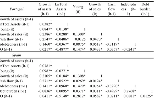
Let now turn to the model for firms growth, which is estimated through a GMM- system.45 Table 5.4 shows the mutual contemporaneous correlation coefficients among the regressors and the dependent variable.46 Cash flow and growth of sales exhibit a positive correlation with firm growth
above 20%. Consistently with previous analysis, indebtedness is weakly but positively related with firm growth, while debt burden coefficient is negative. Likewise, FO is negatively related to firm size, i.e. the natural logarithm of real total assets, firm growth and the availability of cash flow, while it is positively related with debt variables.
Table 5.4 Correlation matrix
Full sample Growth of assets (it-1) LnTotal Assets (it-1)
Young (it) Growth of sales (it) Cash flow (it-1) Indebted ness (it-1) Debt burden (it-1) Growth of assets (it-1) 1
LnTotalAssets (it-1) 0.0550* 1
Young (it) 0.0752* -0.0642* 1
Growth of sales (it) 0.2199* 0.0009 0.1089* 1
Cash flow (it-1) 0.2551* -0.0894* 0.0211* 0.0161* 1
Indebtedness (it-1) 0.0808* -0.0393* 0.0983* 0.0443* -0.3513* 1
Debt burden (it-1) -0.1121* 0.0391* 0.0254* -0.0088* -0.5132* 0.2693* 1 FO (it-1) -0.0187* -0.1365* 0.0825* -0.0045* -0.1011* 0.1703* 0.0345* Note: The table reports the contemporaneous Pearson correlation coefficients among the variables of interest. Growth of assets is the difference between the natural logarithm of real total assets for two subsequent years. Young is a dummy variable which takes value 1 if the firm has less than 6 years. Growth of sales is the difference between the natural logarithm of real sales for two subsequent years. Cash flow is the sum of the per-period profit/losses and depreciation, scaled on the total assets at the beginning of the period. Indebtedness is the ratio between total debt and total assets. Debt burden is the ratio between interest paid and EBITDA. FO is the predicted probability of having financing obstacles. The * indicates that coefficients are significant at the 5% level. Source: AMADEUS Bureau van Djik Electronic Publishing and own calculations.
In Panel A of Table 5.5, I consider the classical LPE equation, equation (3). I always control for year and sectoral effects. The results clearly reject LPE in Germany and in Portugal, since current size affect firms growth. In France, Italy and Spain the validity of the instruments is not confirmed by the tests. However, the aim of the paper is to investigate the determinants of firms growth and to check whether the probability of facing financing obstacles negatively affects firms growth. Thus, I estimate three specifications of the augmented LPE model, equation (4). In particular, in Panel B I add to the standard LPE equation the dummy young and firms profitability, in Panel C I also consider indebtedness and FO, and in Panel D I include an additional measure of