View of Modelling comovements of economic time series: a selective survey

MODELLING COMOVEMENTS OF ECONOMIC TIME SERIES: A SELECTIVE SURVEY

M. Centoni, G. Cubadda

1. INTRODUCTION

A large body of literature in time series analysis is dedicated to modeling co-movements amongst multiple economic variables. The word comovement has been used in different meaning: even the spelling is uncertain, in most cases it can be found co-movement. In the present paper, comovement can be defined as “move together”, that is as movement that several series have in common. Comovements are often studied using correlation (e.g. Forbes and Rigobon, 2002; Imbs, 2004; Bax-ter and Kouparitsas, 2005): some extension are, among others, dynamic correlation of Croux et al. (2001) and the concordance index of Harding and Pagan (2006). However, economic time series have many characteristics such as trends, cycles, sea-sonality, serial correlation, and so on. Then it is important to consider these proper-ties when analyzing comovement. To this respect (Vahid and Engle, 1993, pag. 341):

comovement among time series indicates existence of common components. A well known example of comovement is cointegration (Engle and Granger, 1987; Johansen, 1988; Stock and Watson, 1988): a group of series that possess stochastic trends is cointegrated when its element share some common stochastic trends. Due to the importance of cointegration for empirical research, most of the intuitions behind that were extended to the analysis of comovements among stationary series. Gourieroux and Peaucelle (1988) first extended the concept of cointegration to stationary time series and called this codependence: a group of variables are codependent if there exists a linear combination of them that pos-sesses shorter memory than individual series. Later, Vahid and Engle (1997) show that codependence implies common short-run components. Another example of linear combinations of stationary variables that have lower order dynamics than the individual series is the scalar component model (SCM) of Tiao and Tsay (1989), that studied this type of structure in a multivariate ARMA model. These ideas were further developed and formalized in a series of paper by Engle and Kozicki (1993) and Vahid and Engle (1993). Engle and Kozicki (1993) considered features that satisfy the following axioms:

1. The vector series X has (does not have) the feature if any non-singular lin-t

ear transformation of X still has (does not have) such feature; _t

2. If two n-vector time series Y and 1t Y do not have the feature then 2t

1 2

(Yt Yt) does not have the feature;

3. If Y does not have the feature but _t X has the feature then _t (Y_t X_t) has the feature.

Then, any dynamic property of the data could be viewed as a special case of feature: for example, series with stochastic trends satisfies all axioms. As pointed out by Engle and Kozicki (1993) a linear combination of two series that both have the feature does not necessarily posses the feature. This is the most interest-ing case, and to this issue Engle and Kozicki gave particular attention by the fol-lowing definition:

Definition 1: A feature, which is present in each of a set of series, is said to be common to those series when there exists a nonzero linear combination of these series that does not have the feature.

It follows that cointegration is a special case of common features. Nowadays, there is a huge collection of special cases of common features. A comprehensive, although still partial, list includes: serial correlation (Engle and Kozicki, 1993; Va-hid and Engle, 1993), when a linear combination of serially correlated series is white noise; cotrending (Chapman and Ogaki, 1993), when a linear combination of trend-stationary time series no longer display deterministic trend; common volatility (Engle and Kozicki, 1993; Engle and Susmel, 1993), when a linear com-bination of ARCH series eliminates the ARCH effects; common seasonality (Engle and Hylleberg, 1996), when a linear combination of seasonally integrated series is nonseasonal; co-breaking (Hendry, 1996), when a set of series appear subject to structural breaks but a linear combination of variables does not display the breaks; codependent cycles (Vahid and Engle, 1997), when a linear combina-tion of a group of variables has shorter memory than the individual series; nonlinearity (Anderson and Vahid, 1998), when the conditional expectation of each element of a vector time series is nonlinear w.r.t. the conditional vector but there exist a linear combination of them whose conditional expectation is linear w.r.t. the conditional vector; common seasonal cycle (Cubadda, 1999), when there exists a linear combination of seasonal differenced series which follows an MA process of low order; common panel structure (Hecq et al., 2000), when there is a linear combination of the variables in a panel data which is white noise for all in-dividuals of the panel; nonlinear cotrending (Bierens, 2000), when a linear combi-nation of the components of a set of stationary time series around nonlinear de-terministic time trends is stationary around a linear trend or a constant; polyno-mial serial correlation (Cubadda and Hecq, 2001), when there exists a polynopolyno-mial combination of serially correlated time series that is white noise; long-run pure variance (Engle and Marcucci, 2006), when the conditional variances of a

collec-tion of assets all depend upon a small number of variance factors; non-innovacollec-tion (Paruolo, 2006), when a linear combination of a demeaned autocorrelated process is an innovation process, i.e. non predictable; weak serial correlation (Hecq et al., 2006), when a linear combination of serially correlated series adjusted for long-run effects is white noise; periodic correlation (Haldrup et al., 2007), when a lin-ear combination of periodic series is not periodic.

Instead of analyzing separately different properties of a time series, it could be useful to develop a unifying framework in order to contemporaneously analyzing several properties. Cubadda (2007) made this with respect to different forms of common cyclical features, introducing the notion of weak polynomial serial corre-lation which encompasses most of the existing formucorre-lation.

From a statistical point of view, comovements imply a reduction to a more parsimonious structure such as common factor representation (see, inter alia, Gonzalo and Granger, 1995), that can be estimated by reduced rank regression techniques (Anderson, 1984, 1999) with considerable efficiency gain (Vahid and Issler, 2002). Let Yt be an n-vector time series such that

t t t

Y Bf  e

where (n−s) common factors ft have the feature and et does not have the

fea-ture. Consider a s−vector  such that  B , then 0  Y_t does not have the fea-ture.

Comovements among time series are often predicted by economic theory. For example, in King et al. (1988) the solution of their macro model implies that out-put, consumption and investment have a common trend and a common cycle. The common stochastic trend is generated by an integrated productivity shock, while the deviation of capital stock from its steady state value determines the transitional dynamics of output, consumption and investment. Other example is Campbell (1987) where the saving path implies that disposable income and con-sumption cointegrate (Issler and Vahid, 2001). However, it could happen that ob-served comovements are in contrast with the theoretical model, and some efforts are toward reconciling the model with the data: as an example, in the DSGE model of Justiniano et al. (2010), an extension of the well known model of Chris-tiano et al. (2005), investment shocks are the driven forces of fluctuations over the business cycle. In this model, however, consumption typically falls after an investment shock. This finding is in contrast with the observed business cycle comovement between consumption and investment. Khan and Tsoukalas (2011) try to solve this “comovement problem” introducing some modifications to tradi-tional DSGE model.

The large body of literature on comovement obviously forces one to contain the discussion to some arguments: see Urga (2007) for a recent survey. Then, the plan of the rest of the paper is as follows. After introducing the general concept in Section 2, Section 3 discusses the implications of the presence of common trends in I(1) processes. Section 4 presents as different types of common

season-ality as many seasonal patterns. Section 5 deals with alternative notions of com-mon cycles. Section 6 takes into account the consequences of the presence of common features with respect to univariate representation of time series models. Finally, Section 7 concludes.

2. COMMONFEATURESINECONOMICTIMESERIES

The main idea is that a small number of unobserved components posses a given feature and transmit it to a larger set of economic time series. It is then possible to combine such time series in order to cancel the influence of these un-observed components, thus removing the common feature from the data. Re-duced-Rank Regression (RRR) (Anderson, 1984) is often the statistical solution to the inferential problem.

Let Y be a stationary n-vector time series such that t

t t t t

Y X Z  

where X and t Z are, respectively, vectors of k and m variables, t   , and 0 t

are i.i.d. Nn(0, ) errors that are independent from both X and t Z . Both t X t

and Z may contain (linear functions of) lags of t Y . t

Let us assume that:

1. Variables X posses the feature of interest whereas variables t Z don’t. t

2. There exists a n×s (s<min{n,k}) full-rank matrix  such that  Yt do not

posses the feature. Then, it is said that variables Y have s Common Features. t

In view of the above assumptions we get

t t t Y Z     that is equivalent to 0     _ 

where _ is a n×(n−s) full-rank matrix such that   _ , and 0  is a k×(n−s)

matrix.

If n>k, the matrix  _{has not full column-rank, then there exist (n−k) “trivial”}

CF. Hence, let us also assume that s<n≤k, so the matrix  has full-rank as well.

2.1 Common Features & Reduced Rank Regression

The cofeature matrix  and the coefficient matrix  are usually obtained by means of RRR. The procedure can be summarized as follows:

1. Regress both Y and t X on t Z and obtain the partial regression model t t t t y x   where yt Yt E Y Z( | )t t , xt Xt E X Z( t| )t ,   xx xy1 , and var t yy yx xy xx t y x                 

2. Solve the following maximization problem

1 1 arg max xx n yx xx xy yy                 _{  }     _{ }         s.t. 1yy 

Then we get the solution 1/2 1 yy 1

 _  _{, where} j

 (j=1,…,n) is the eigen-vector associated to the j-th largest eigenvalue _j (₁₂  ... n) of the symmetric, semi-positive definite matrix

1/2 1 1/2 yy yx xx xy yy         Note that 2_{( | )} t t

R y x _{, where}   , is maximized for   and 1 1 1 xx xy 1  _{  }  _since 1 1 1/2 1 1/2 1 1 1 1 1 1 yy xx yy yx xx xy yy                    

3. Solve the following maximization problem 1 2 arg max n yx xx xy yy                  _{ }     s.t. 1 1 0 yy yy        

We get the solution 1/2 2 yy 2  _  Note that 2 2 2 2 ( t| t) R y x  where  1 2 xx xy 2  _{ }  _{. Moreover,} 2 1 2 ( t| t) 0 R y x _{ since} 1/2 1 1/2 2 xy 1 2 yy yx xx xy yy _  __ _{   }  _,

4. In general, we have that 1/2

j yy j

 _  _{is the solution of:} 1 arg max n yx xx xy j yy                  _{ }     s.t. 1 0 j yy j i yy j          for i j 2,...,n. Moreover, 2_{( | )} for 0 for j i t j t i j R y x i j    _{ }    , where 1 j xx xy j  _{ }  _.

5. Since   _{ then so is} 0   _xx , that implies that n s 1 ... n  , 0

then the cofeatures matrix  is obtained (up to an identification matrix) as follows

1 ( n s ,..., n)

   _{ } 

6. Since 1 ... n s  , the coefficient matrix 0  is obtained (up to an iden-tification matrix) as follows

1

( ,..., _{n s})

    _

7. Finally, the loading matrix _ is given by the regression coefficients of yt

on xt.

It is worth remarking that the eigenvalue problem

1/2 1 1/2

yy yx xx xy yy  

  

      (1)

is equivalent to finding the roots of the equation:

1 1

yy yx xx xy 

 

     (2)

with the normalization _yy  . 1

The solution of the above problem (equivalent to RRR) is known in statistics as partial canonical correlation analysis between Yt and Xt conditional to Zt,

and it is denoted by CanCor( ,Y X Zt t| )t

2.2 Common Features & Reduced Rank Regression: Statistical Inference

Under the assumption that ( , )y xt   are normally distributed, RRR provides t

ML inference on  and  (Anderson, 1984). The LR test statistic on the exis-tence of s Common Features is:

1 ˆ LR( ) n ln(1 i) i n s s T      



where ˆi is the i-th largest eigenvalue of the sample matrix ˆyy1/2   ˆyx xx xyˆ1ˆ ˆyy1/2.

Under proper regularity conditions on the variables X and t Z the test statistic t

(3) is distributed 2

LR( )s d [ (s k n s  )].

The ML estimator of the cofeatures matrix  is obtained (up to an identifica-tion matrix) as follows

1 ˆ _{(ˆ ,..., ˆ )} n s n    _{ }  , where _{ˆ ˆ} 1/2_ˆ j yy j  _  _{and ˆ} j

 (j 1,..., )n is the eigenvector associated to the j-th

largest sample eigenvalue ˆj.

The ML estimator of the coefficient matrix  is obtained (up to an identifica-tion matrix) as follows

1 ˆ _{( ,...,}ˆ ˆ_{n s)}     _ , where _{ˆ ˆ} 1_{ˆ ˆ} j xx xy j  _{ }  _.

The ML estimator of the loading matrix _ is finally obtained by the regres-sion coefficients of y on t ˆxt.

The degrees of freedom of the test statistic (3) are obtained as follows. Under 1

H the matrix  is composed by n×k elements. Under H we have that 0  _,1 _,2 ( _{) ( ) ( ) ( )} ( : ) k n s _{n s n s n s s}   _ _   _{    }  .

Without loss of generality, we assume that ,1 has full-rank. Then we can write

1 ,1 ,1

where  ( ,Is ,2). Hence, the matrix  is composed by (n−s)×(s+k) ele-ments. It follows that under H 0 s(k−n+s) restrictions are imposed.

3. COMMON TRENDS

Macroeconomic time series often display a clear trending behavior, and stan-dard unit-root tests suggest that series need to be treated as processes integrated of order 1 (I(1) for short) rather than trend stationary. However, linear combina-tions of such series do not show similar patterns, instead appears to be stationary: this is what is intended by cointegration. Cointegration introduced by Granger (1981) has became one of the most widely used concept in time series economet-rics, due to the straightforward economic interpretation of the cointegrating rela-tions as long-run equilibrium relarela-tionships. Comovement arises by the presence of common stochastic trends in the series, that are removed by the cointegrating relations. It is worth noting that if the non stationary behavior is due to presence of deterministic rather than stochastic trend, we refer to a stationary linear com-bination of these series as cotrending relations (Chapman and Ogaki, 1993) or nonlinear cotrending relations, if non stationarity is due to nonlinear deterministic time trends (Bierens, 2000). The cointegrated vector autoregressive (VAR) model pioneered by Johansen (1988, 1996) is the most commonly used econometric tool: see Juselius (2006) for the use of cointegrated VAR models in macroeco-nomic empirical research. In what follows we briefly review this model and de-scribe the procedure to determine the number of cointegrating relations.

3.1 Cointegration: Assumptions & Definition

A n-vector of time series { ,y tt 1,..., }T is generated by the VAR(p) model:

( ) t t t

A L y D  (4) 

where ( ) p₁ i

n _i i

A L  I



i.i.d. Nn(0, ) errors. Assume that elements of y are, at most, I(1), denoted by t t

y ~I(1). By expanding ( )A L on 0 and 1, we rewrite (4) as

1 ( )L y_t D_t A(1)y_t _t      (5) where ( )L In _ip₁1 iLi  

  





must be stationary as well. Three possible cases can arise:

1. (1) 0A  , means that all the elements of y are I(1) and do not cointegrate, t

2. rank[ (1)]A  , then all the elements of n y are I(0); t

3. rank[ (1)]A  , then (1)n A  , where  and  are full-rank

n×r-matrices 1,...,r n and it follows 1 y_t~I(0). Series y are cointegrated _t

of order (1,1), y ~CI(1,1), the space spanned by t  is the cointegration

space.

If variables cointegrate, we can rewrite the model (5) in his Vector Error Cor-rection Model (VECM) representation:

1 ( )L yt Dt yt t

     (6)

where series y_t react to previous stationary deviations from the equilibria. Series

t

y admit the following Wold representation:

( ) t t t y D C L     (7) where Dt C L( )Dt, and C L( ) In _{i 1}C Li i    





By expanding ( )C L on 1 and integrating both sides of the above equation, we

get the multivariate Beveridge-Nelson representation (Beveridge and Nelson, 1981): 0 1 (1) ( ) t t t j t j y y D C  C L        







y share the following (n−r) common stochastic trends: 1 t t j j   _   



Note the analogy between (8) and the common factor representation of the in-troduction: ( )C L _t does not have the feature, while t has the feature, and the

(n−r) common stochastic trends are removed by the cointegrating vectors, since 1

( ) 0

   _{    }  _{ . For alternative identifications of the common trends see} Gonzalo and Granger (1995) and Johansen (1996) among others.

3.2 Cointegration: ML Inference

In order to determine the number of cointegrating relations and consistently estimate parameters of the VECM (6), Johansen (1988, 1991, 1996) proposed to resort to RRR in a Gaussian ML framework. In particular, the number of cointer-grating relations is based on the solution of the following problem:

1 1 1 CanCor , _... t t t t t p D y y y y               _{ }  _{ }  _{ }    _{ }   ,

and then conducts a LR test for H rank[A(1)]=r vs 0 H rank[A(1)]=n using the 1 test statistic: 1 ˆ ln(1 ) n j j r T    



where ˆj is the j−th largest squared canonical correlation. If the null hypothesis

is not rejected, the ML estimator of  are the r eigenvectors associated with the r largest eigenvalues ˆ₁,...,ˆ_r.

Note that when D_t is a constant, the test statistic Q(r|n) converges weakly in distribution to 1 1 1 1 0 0 0 tr d ( ) ( )B u F u F u F u u( ) ( )d F u B u( )d ( )   _{ }   _{  }            







where {}tr  denotes trace, B(u) is the standard Brownian motion of dimension

(n−r), and

1 0 ( ) ( ) ( )d

F u B u 

_

Moreover, when D is not constant (linear trend, step dummy, ...) in the esti-_t

mated model, F(u) has a different formula. However, the limit distribution of the test statistics does not depend on  (Johansen, 1991).

The ML estimator of , ˆML, is T−consistent and its limit distribution is

mixed-Gaussian, so tests on  are asymptotically _2 _{but the exact distribution} of (normalized) ˆ_ML has Cauchy-like tails (Phillips, 1994).

Finally, the remaining parameters in VECM (6) are estimated by OLS after fix-ing the matrix  to its estimated value, see Johansen (1996) for further details.

4. COMMON STOCHASTIC SEASONALITY

Most of economic time series display a seasonal pattern that evolves in a sto-chastic fashion (Hylleberg et al., 1993). Focusing, for simplicity, on quarterly time series, variables y are seasonally integrated of order 1 (Hylleberg et al., 1990) if t

4yt  is stationary, where 4 4 (1 L )    . Notice that 2 4

frequency 0 frequency frequency /2 (1 L) (1 L) (1 L )

 

  _{  } _ _{ ,}

which allows for three diverse kinds of cointegration relations:

1. Cointegration at frequency 0, if a linear combination of 2

1,t (1 )(1 ) t

y  L L y is stationary.

2. Cointegration at frequency , if a linear combination of 2

2,t (1 )(1 ) t

y  L L y is stationary.

3. Polynomial cointegration at frequency /2 , if a linear combination of 3,t (1 )(1 ) t

y  L L y and its lags is stationary.

4.1 Seasonal Cointegration: Assumptions & Definition

Let { ,y tt 1,..., }T be an n-vector of time series generated by the following VAR(p) model:

( )L yt Dt t

   (9)

where ( ) L is a p-order polynomial matrix, t are i.i.d. Nn(0, ) , and D is a t

deterministic kernel.

Assume that elements of y are, at most, I(1) at frequencies 0, t  , and /2 .

By expanding Π(L) on 0, ±1 and ±i, we rewrite the VAR (9) as

4 1 1, 1 2 2, 1 , 1 , 1 ( )L yt Dt y t y t   y t   y t t         where ( ) p ₁4 j n j j L I _ L   





    and C denotes the complex conjugate of a com-plex matrix C.

Since 4yt~I(0), then 1 1,y t, 2 2,y t, and  y ,t must be stationary as well.

If the series are cointegrated of order (1,1) at frequencies 0, , and /2 , the VAR(p) model may be rewritten in the following Complex VECM (CVECM)

4 1 1 1, 1 2 2 2, 1 , 1 , 1

( )L y_t D_t  y _t  y _t  _{   }y _t  _{   }y _t _t

where _j and _j are n r -matrices with rank equal to _j r for j=1,2, and _j _ and

_ are complex n r -matrices with rank equal to₃ r , see Cubadda (2001) and ₃

Cubadda and Omtzigt (2005).

Notice that four cointegrating relationships are present in the CVECM. In-deed, ₁ and ₂ are, respectively, the cointegration matrices at frequencies 0 and

, whereas the conjugate complex cointegration matrices  and _ _ are re-spectively associated with frequencies

2  and 3 2  .

Since complex valued cointegration vectors are not amenable to economic in-terpretation, we rewrite the complex VECM in the following Seasonal VECM (SVECM) 4 1 1 1, 1 2 2 2, 1 4 3 3 4 3, 1 ( )L yt Dt  y t  y t (  L)( L y) t t          where 3 4 3 4 1 ( )( ) 2 i i

 _{ }    , see Lee (1992) and Ahn and Reinsel (1994). It is worth remarking that the SVECM exhibits a real but polynomial cointe-gration vector ( )L 34L for the annual frequency. Further, the CVECM is more convenient than the SVECM for statistical inference because the cointe-gration restrictions at the various frequencies imply the usual reduced-rank struc-ture of the ’s matrices.

4.2 Seasonal Cointegration: ML Inference

In order to determine the number of seasonal cointegrating relations, Hylle-berg et al. (1990) suggest a two-step procedure after having appropriately filtered the series. Since this procedure need pretesting for seasonal root, Cubadda (2001) proposed a more general procedure that do not require any prior knowledge about seasonal integration and allows to test for seasonal cointegration at any col-lection of frequencies. The procedure can be summarized as follows. Regress

4 yt

 , y1, 1t , y2, 1t , and y , 1t on (Dt,4yt1,...,4yt p 4) and take respectively the residuals R , 0,t R , 1,t R , and 2,t R,t. These residuals asymptotically satisfy the

following equation

0,t 1 1 1, 1t 2 2 2, 1t ,t ,t t R  R _  R _  _{  }R  _{  }R  

Since the processes R , _1,t R , _2,t R_,t, and R,t are mutually asymptotically

un-correlated, we can ignore reduced rank restrictions at the frequencies different from the one of interest.

Hence, the (concentrated) ML solution is obtained by solving

0, 1, 2, , , CanCor{R t,R Rt t,Rt,Rt}

for cointegration analysis at frequency 0, and

0, 2, 1, , , CanCor{R _t,R _t R R_t, _t,R_t} for cointegration analysis at frequency .

Johansen and Schaumburg (1998) showed that the (concentrated) ML solution for cointegration analysis at frequencies

2  and 3 2  cannot be obtained by RRR. However, the solution of

0, , 1, 2, , CanCor{R t,R R Rt t, t,Rt}

provides asymptotically optimal inference for cointegration at frequency 2



(Cu-badda, 2001).

It is worth remarking that small sample improvements may be obtained by es-timating the cointegration vectors jointly at the zero and seasonal frequencies (Cubadda and Omtzigt, 2005).

5. COMMON CYCLES

As we have seen in Section 3, a set of I(1) cointegrated time series share some common stochastic trends. However, detrended economic time series often dis-play clear evidence of comovements (Lucas, 1977), which cannot be due to coin-tegration, thus suggesting the presence of common cycles. If this is the case, we expect that there exists linear combination of cyclical series the are not cyclical. This Common Cyclical Features [CCF] (Engle and Kozicki, 1993; Vahid and Engle, 1993) can be interpreted as short-run equilibrium relationships, similarly to the interpretation of the cointegrating relations as long-run equilibrium. Indeed, common cycles appear in many theoretical economic models. For examples, in models of aggregate consumption behavior as discussed in Vahid and Engle (1993) and Issler and Vahid (2001), the proportion of total income that accrues to “myopic” individuals (Campbell and Mankiw, 1990), that is, individuals that con-sume their income entirely in every period, or excess sensitivity of consumption to current income (Flavin, 1993), provide that first differences of I(1) consump-tion and income share a common cycle. Note that in the consumpconsump-tion theory of Hall (1978) consumption and income share only a common stochastic trend. In real business cycle models as in King et al. (1991) consumption, investment and income have a common cycle due to the fact that transitional dynamics of the system is a function of the deviation of the capital stock from its stationary value: see Issler and Vahid (2001). As another example, in the real business cycle model for sectoral output à la Long and Plosser (1983), as in Engle and Issler (1995), common cycles depend on the propagation mechanisms through the restrictions

on the production function, i.e. technological constraints. Hence, CCF implies restrictions on the VAR parameters that have meaningful implications for the short-run components of an I(1) vector time series, that can be estimated by the RRR techniques of Section 2.

5.1 Alternative notions of Common Cyclical Features

Let us start with the multivariate Beveridge and Nelson (1981, BN) cycles of series y : t ( ) t C L t     , where (1) ₀1 1 t t C t  





As showed in Section 3, from the Granger representation theorem (Engle and Granger, 1987) we know that the presence of cointegration is equivalent to the existence of (n−r) common stochastic trends since  t  . The analysis of 0 CCF’s is instead concerned with reduced-rank restrictions on the VECM parame-ters that have interesting implications on the cycles _t.

However, differently from cointegration, there is not a unique notion of com-mon short-run components. Indeed, also the degree of synchronicity of the common cycle plays a role in the definitions. Alternative notions of CCF impose differing reduced-rank structures to the VAR. Let us briefly review various form of CCF starting with the seminal notion proposed by Engle and Kozicki (1993). 5.1.1 Serial Correlation Common Feature [SCCF]

Series yt have s (s<n) SCCF’s iff there exists an n×s matrix S with full

col-umn rank such that the VECM (6) can be rewritten into the following RRR model 1 1 1 ( , ,..., ) t t S S t t t p t y D  _ y_ y_ y_{ }            (10)

where S is an (np−n+r)×(n−s) matrix with full column rank (Engle and Kozicki,

1993). Since Syt SDt  S t , there exist s linear combinations of series yt

that are unpredictable from the past, i.e. they are innovation processes. Since 0

S t

   , there exist (n−s) common cycles in series y (Vahid and Engle, 1993) _t

that are perfectly synchronized, as a results the impulse responses functions are exactly collinear. However, one observes that due to technical reasons (e.g., sea-sonal adjustment) as well as economic reasons (e.g., adjustment costs, labor mar-ket rigidities), the hypothesis underlying SCCF is sometimes too strong, since SCCF is not able to detect the existence of non-contemporaneous cyclical co-movements (Ericsson, 1993). Then, some less restrictive variants of the SCCF have been introduced in the literature, which we will review in turn.

5.1.2 Polynomial Serial Correlation Common Feature [PSCCF]

Cubadda and Hecq (2001) propose the notion of polynomial serial correlation common features as a measure of non-contemporaneous cyclical comovements. Non-synchronous common cycles arises, for example, in economic model of consumption with several types of consumer goods as, among others, in Vahid and Engle (1997) and Schleicher (2007): it is shown that the maximization prob-lem of the representative agent implies a unsynchronized common cycle (code-pendent cycle) in the consumer goods vector.

By definition, series yt have s PSCCF’s iff there exists an n×s matrix P with

full column rank such that   P 1 , and the VECM (6) can be rewritten into the 0 following partial RRR model

1 1 ( 2,..., 1, 1 )

t t t P P t t p t t

y D y_  _  y_ y _{ } y_ 

           , (11)

where _P is an (np−2n+r)×(n−s) matrix with full column rank (Cubadda and Hecq, 2001).

In order to interpret the notion of PSCCF, Cubadda and Hecq (2001) show that there exists a first-order polynomial matrix ( ) L _P _PL such that

( )L yt P Dt P t

     .

Hence, PSCCF requires that there exists a first-order polynomial matrix ( ) L

such that ( ) L yt is white noise. The presence of PSCCF has an interesting

im-plication for the BN cycles of series y : indeed, since t ( )L  t 1C(1)t, the

same PSCCF relationships cancel the dependence from the past of both the first differences and cycles of series y . t

5.1.3 Weak Form of Serial Correlation Common Feature [WF]

In the above definitions of CCF, the number of SCCFs or PSCCFs, s, cannot exceed the number of common trends (n−r). In order to remove this restriction, Hecq et al. (2006) proposed the notion of weak form of SCCF: series yt have s

WF’s iff there exists an n×s matrix W with full column rank such that  W  , 0

and the VECM in (6) can be rewritten into the following partial RRR model

1 ( 1,..., 1)

t t t W W t t p t

y D y_  _  y_ y_{ } 

        

where W is an (np−n)×(n−s) matrix with full column rank (Hecq et al., 2006).

In order to uncover interesting implications of the WF for the BN cycle, Cubadda (2007) shows that there exists a first-order polynomial matrix

( ) ( ) W L W In WL      such that ( ) W L yt W Dt W t      .

As consequence, since W( )L  t W (In C(1))t, the same WF relationships

cancel the dependence from the past of both the cycles and linearly detrended levels of series

y

5.1.4 Weak Form of Polynomial Serial Correlation Common Feature [WFP]

A limitations of the above methods for cyclical features analysis is that they cannot handle the possible coexistence of differing types of reduced-rank restric-tions in the same vector. In order to overcome this limitation, Cubadda (2007) introduced the notion of weak form of PSCCF, which encompasses most of the existing formulations: series yt have s WFP’s iff there exists an n×s matrix F

with full column rank such that  F  , 0   F 1 , and the VECM in (6) can be 0 rewritten into the following partial RRR model

1 1 1 ( 2,..., 1)

t t t t F F t t p t

y D y_ y_  _  y _ y_{ } 

          

where F is an (np−2n)×(n−s) matrix with full column rank.

The WFP requires the existence of a second-order polynomial matrix 2 1 1 ( ) ( ) F L F In FL FL        such that ( ) F L yt F Dt F t      .

An important implication of the WFP is that the polynomial matrix F( )L transforms the BN cycles t into a process with shorter memory, since

( )

F L t

  ~VMA(1). 

5.2 Common Cyclical Features: ML Inference

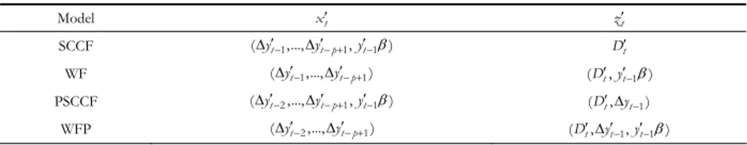
In order to determine the number of CCF’s and consistently estimate parame-ters of the VECM (6), it is standard practice to resort to RRR (i.e., Engle and Kozicki, 1993; Vahid and Engle, 1993; Cubadda and Hecq, 2001). In particular, let CanCor{y x zt, | }t t denote the partial canonical correlations between series

t y

 and x conditional on t z . ML inference on the various forms of common t

features is obtained by solving CanCor{y x zt, | }t t for proper choices of the

variables x and t z , as in Table 1A. t

TABLE 1A Canonical correlations and CCF’s

Model xt z t

SCCF (yt1,...,yt p 1,yt1) Dt

WF (yt1,...,yt p 1) (D yt , t1)

PSCCF (yt2,...,yt p 1,yt1) (Dt , yt1)

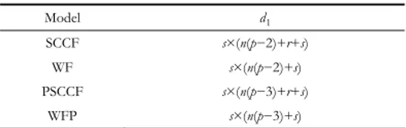
Let ˆi denote the i-th smallest squared partial canonical correlation for

1,...,

i n. Under the null that s common features of a given form exist, the test statistic 1 1 ˆ ln(1 ) s i i LR T    



 as detailed in Table 1B (see, inter alia, Velu et al., 1986; Anderson, 2002).

TABLE 1B Tests for common features

Model d1 SCCF s×(n(p−2)+r+s) WF s×(n(p−2)+s) PSCCF s×(n(p−3)+r+s) WFP s×(n(p−3)+s) Moreover, let ˆ y i  and ˆx i

 respectively denote the partial canonical coefficients of yt and x associated with t ˆi . Optimal estimates of both the common

fea-tures vectors and (partial) RRR coefficients are then obtained as described in Ta-ble 2 (see, inter alia, Velu et al., 1986; Ahn and Reinsel, 1988).

TABLE 2

Estimators of the common features vectors and RRR coefficients

Model ₍ˆ₁y_,...,ˆ y₎ s   (ˆsx1,...,ˆnx) SCCF ˆS ˆS WF ˆW ˆW PSCCF ˆP ˆP WFP ˆF ˆF

Finally, the remaining parameters of the various RRR models are estimated by OLS after fixing the matrices  ’s to their estimated values.

5.2.1 Serial Correlation Common Feature when n is large

ML inference discussed so far may perform poorly with high-dimensional sys-tems, because inversions of large variance-covariance matrices are required. Hence, there exist problems of size and power in usual tests when the number of series, n, and the number of lags in the VAR, p, are large relative to the sample size, T. Cubadda and Hecq (2011) propose an alternative strategy to detect the presence of common cyclical features, SCCF in particular: they show that a Partial Least Squares (PLS) approach can be used to test and impose a RRR structure to

“medium” n systems VAR’s even in cases when canonical correlation analysis is not feasible due to a lack of degrees of freedom. The idea is to replace the condi-tion that a linear combinacondi-tion of variables must be orthogonal to the past with the one of absence of autocorrelation (see, e.g., Lucke, 1994). To illustrate the idea, consider that equation (10) implies

1 E(S y wt| t ) 0 (12) where 1 ( 1 , 1,..., 1) t t t t p w_  y_ y_ y_{ }  (13)

However, when n or p are large relatively to the sample size T, it is convenient to resort to a weaker orthogonality condition, namely

1

E(Si yt|[ytSi,...,yt p Si  ] ) 0  , i1, 2, , (14) s where S [ S1, S2,...,Ss]. This drastically decreases the number of restrictions

to be imposed under the null hypothesis, thus making a test for (an implication of) SCCF feasible even when canonical correlation analysis [CCA] is not. In order to detect SCCF in high-dimensional systems, Cubadda and Hecq (2011) propose to test for this condition by means of univariate tests for no serial correlation of each   Si yt having fixed S to a consistent estimate of a base for the SCCF

space. However, it remains the problem of estimating common feature vectors. Cubadda and Hecq (2011) use a PLS approach instead of CCA that works well even in cases when CCA is not feasible due to a lack of degrees of freedom (both in simulations and empirical applications). PLS, introduced by Wold (1985), are a family of multivariate techniques with the aim of maximizing the covariance be-tween linear combinations of two variable sets, see, e.g., Rosipal and Kraemer (2006) for a recent survey.

From Section 2.1 and 5.2, we know that the CCA estimator of SCCF is

1

ˆCCA _[ˆCCA_,...,ˆCCA_]

S s

    ,

where ˆCCA i

 is the eigenvector associated with the i-th smallest eigenvalue of the matrix _{ˆ ˆ}1 _ˆ 1_ˆ yy yw ww wy       , where ˆ_yy E( y y_{t t}), ˆ_ww E(w w_t_{1 t}₁) and 1 ˆ _{E( )} yw y wt t     .

The PLS estimator of the SCCF matrix S is

1 ˆPLS _[ˆPLS_,...,ˆPLS_] S s     (15) where ˆPLS i

ei-genvalue of the matrix _ˆ 1_{ˆ ˆ} 1_ˆ

yy yw ww wy

D D  , with D and yy D are diagonal matrices ww

having the diagonal elements of, respectively, _yy and ww.

Note that, since PLS require to invert diagonal matrices only, this method can provide estimates of S (up to an identification matrix) that are less disperse and

more numerically stable than the CCA estimator when the dimension of w ap-t

proaches the sample size T.

To consistently estimate the factor weights _S, let’s assume that the columns of the matrix _S are equal to (n−s) distinct eigenvectors of the matrix 1

ww ww D , then we get 1 1 1 ww wy yy yw S S yy yw D_ D_{ } V__D_

where V is the diagonal matrix of the (n−s) eigenvalues of the matrix Dww ww1

that are associated with the eigenvectors S, which implies that the matrix S

lies in the space generated by the eigenvectors associated with the positive eigen-values of the matrix 1 1

ww wy yy yw

D D .

In order to test for the presence of SCCF in systems where n×p is large, Cu-badda and Hecq (2011) consider tests for the null hypothesis that   Si yt is a

white-noise for i1, 2,...,s as in (14). In particular, we look at the Box-Pierce test statistic 2 , , 1 ˆ k j i i j l l Q T r  







and et ij,  ˆSij yt for j CCA PLS , and i 1, 2,... .s The test statistic Q fol-ij

lows asymptotically a 2 ( )k

 distribution under the null. However, one should con-trol the overall size of the test when applied for different values of s. Cubadda and Hecq (2011) propose two different strategies to solve this problem: using a Bonferroni correction to fix the overall significance level of the s tests computing

max( )

j j

s i

and confronting it with the critical level at

s



% in the 2 ( )k

 ; or, based on Cu-badda et al. (2008), testing for the null of no autocorrelation on the aggregate

, ₁ ,

s

j j

t s _i t i

a 



6. COMMON FEATURES AND UNIVARIATE TIME SERIES MODELS

ARIMA models are still a popular tool for forecasting economic time series, since they often outperform large macro models. Indeed, in macroeconometrics we are typically interested in the interactions between entities, and in order to ac-count for the links between variables we usually resort to a multivariate frame-work (VAR, VARMA, VECM...). However, univariate ARIMA models are also the implied final equations (FEs) of systems such as VARs or VARMAs (Zellner and Palm, 1974). But here a paradox comes: FEs are theoretically non-parsimonious, whereas low order ARIMA models are empirically appropriate. Cubadda et al. (2009) show that VAR models with a reduced-rank structure aris-ing from the presence of common features can give an answer to this paradox.

Let us start by referring to a recent solution to the well-known “autoregressiv-ity paradox”, i.e., multivariate time series models imply highly non parsimonious ARIMA models for individual time-series.

6.1 The Final Equations (FEs) of the VAR

Let us consider the n dimensional VAR(p) (4) ( ) _{t t}

A L y  (16) 

where deterministic terms are omitted for simplicity.

Following Zellner and Palm (1974), the univariate representation of elements of y can be obtained by premultiplying both sides of (16) by ( )t A L adj, the

adjoint matrix (or the adjugate) associated with ( )A L , such that

1 ( )adj det[ ( )] ( )

A L  A L A L  , in order to obtain the Final Equations (FEs)

det[ ( )] ( )adj

t t

A L y A L  , (17)

where det[ ( )]A L is a polynomial of order np and ( )A L adj is matrix polynomial of order (n−1)p.

6.2 Implications of the Final Equations

Equation (17) implies that every FE is an univariate ARMA( *, *)p q although it

is derived from the finite order VAR(p). They have identical autoregressive pa-rameters because det[ ( )]A L is the same of the n equations. Here the paradox: an n-dimensional VAR(p) would imply ARMA(np,(n−1)p) processes, an implication

that is rejected when tested on economic data where one usually finds quite par-simonious ARIMA models.

To illustrate this point, let us assume that n=3 series are generated by the fol-lowing VAR(1): 1 0.5 0.5 0.5 0.25 0.25 0.25 0.5 0.5 0.5 t t t y  y         _   _        where yt (y1t,y2t, y 3t) .

For the above VAR, the FEs are:

3 2 2 2

det[ ( )] 1 0.5A L   L (0.75 2 )  L(1.25  )L , such that individual series follow ARMA(3,2) models.

However, if  , the VAR has reduced-rank structure 0

1 0.5 0.25 [ 1 1 1] 0.5 t t t y y_      _{ }      

which produces the FEs:

1 0.25 0.5 1 0 1 (1 0.75 ) 0.25 1 0 1 0.5 0.5 0.5 t t t L y  _            _  _{ }         .

This implies that the univariate models are parsimonious ARMA(1,1) models with the same autoregressive parameter and cross-correlated errors and a VMA component of FEs with a factor structure.

More generally, Table 3 summaries the reduction of the individual ARMA or-ders due to common features restrictions. As one can see, the presence of com-mon short-run components significantly reduces the order of the univariate ARMA representations. Hence, the existence of CCF’s is a possible, economically meaningful, solution of the paradox.

TABLE 3

Maximum ARIMA orders of univariate series generated by an n-dimensional VAR(p) with s cofeature restrictions

Models AR order I(d) MA order

I(0) np 0 (n-1)p SCCF (n-s)p 0 (n-s)p PSCCF (n-s)p+s 0 (n-s)p+(s-1) C(1,1) n(p-1)+r 1 (n-1)(p-1)+r SCCF (n-s)(p-1)+r 1 (n-s)(p-1)+r PSCCF (n-s)(p-1)+r+s 1 (n-s)(p-1)+r+s-1 WF (n-s)(p-1)+r 1 (n-s)(p-1)+r

It is worth noting that Table 3 provides the maxima ARIMA orders under CCF’s restrictions. However, the orders can be even smaller due to additional re-strictions on the VAR parameters, such as block-diagonal or block-triangular structures.

6.3 Implications of Common Cyclical Features for the VMA component

The presence of short-run comovements has also consequences for the VMA part of FEs. Cubadda et al. (2009) show that in a stationary VAR(p), the existence of s SCCFs implies that in the FEs the VMA coefficient matrices associated with degrees strictly larger than (n−s−1)p have a common right null space that is spanned by _. Hence, it is possible to reduce the order of the VMA component to a degree of at most (n−s−1)p instead of (n−s)p. In particular, when n−1=s, the FEs follow a model that is popular in the macro-panel literature: an homogene-ous AR component and cross-correlated VMA errors having a factor structure. However, in the CF’s framework this model is not a priori assumed but it is an implication of the presence of a (testable) time series property of the data.

In order to clarify this point, it may be appropriate to use an empirical exam-ple. Cubadda et al. (2009) considered the IPIs of Canada and the US. Since they found no cointegration in log levels, a VAR(1) in first differences seemed appro-priate. The estimation by OLS delivers (standard errors in brackets)

  ( 0.088) ( 0.079) ₁ 1 ( 0.102) ( 0.092 ) 0.333 0.273 ln ln 0.265 0.360 ln ln t t t t US US CA CA           _{ }      _{ }        _{  }

Theoretical FEs orders implies an ARMA(2,1) processes. However, SCCF test statistics is in favor of s=1 (p−value=0.31), with the estimated CCF relationship ( ln USt1.05 ln CAt), that is an innovation with respect to the past. Empiri-cal estimation of univariate models gives the following ARIMA(1,1,0)

  1 (0.001) (0.062) 1 (0.001) (0.064 ) ln 0.003 0.554 ln ln 0.004 0.533 ln t t t t US US CA CA          

As expected, AR coefficients are very similar. Moreover, since the estimated cofeature vector ˆ is close to (1: 1) , the variances of VAR residuals are similar, and the correlation of VAR residuals is around 0.65, the previous discussion may explain why the MA(1) components are almost negligible.

6.4 Estimation of the Common AR parameters

As illustrated above, the finding that a set of series have identical autoregres-sive polynomials calls for the estimation of the common AR component that should be preferred to estimating ARMA models for the individual series. Indeed, the univariate parsimonious empirical ARMA( , )p q models can be estimated by i i

ML for each series individually such that

1 1 ˆ ˆ i ˆ i ˆ ˆ p q it i ij it j ik it k it j k y   y _   _     





Instead, imposing the restrictions implied by the VAR is equivalent to using an estimator of the common AR part such that

1 1 ˆ ˆ i ˆ i ˆ ˆ p q it i j it j ik it k it j k y   y _   _     





where ˆ_j is the jth lag order common coefficient to all n which should be pre-ferred to ˆ_ij for individual series.

In order to do so, we have various alternative at hand, such as the mean group estimator (the average of n individual estimators)

1 1 ˆmg n ˆ j ij i n     



and the estimation on aggregates (univariate ARMA for the average of the n se-ries) 1 1 ˆ ˆ ˆ ˆ ˆ p q av t j t j k t k t j k y   y _   _     









and k is the kth lag parameter of the MA part of y . t

Cubadda et al. (2008) have shown by simulation that the best estimator is sim-ply to fit the parsimonious model on aggregates. It is worth noting that the use of this estimator is fine under the null that the FEs are from the same initial VAR

model. However, one could evaluate whether this is also true when we “errone-ously substitute” to the group of variables having common cycles additional se-ries from another group. Cubadda et al. (2009) conducted a Monte Carlo experi-ment and found that the empirical bias increases if one includes series with AR coefficients more distant from the FEs. However, the differences in terms of bias and RMSE decrease as n and T increase.

When we work on the aggregate series, we impose the common autoregressive roots whose estimation can be volatile in individual series. It is worth remarking that due to the factor structure of the VMA component of the FEs, aggregation can reduce the order of the univariate MA components, which are noise in this estimation problem. For instance, in the FEs

1 0.25 0.5 1 0 1 (1 0.75 ) 0.25 1 0 1 0.5 0.5 0.5 t t t L y  _     _       _  _{ }        

pre-multiplication of both sides by (1,1,1) annihilates the VMA component.

7. FINAL REMARKS

The main idea behind this survey was to create a “common thread” between various topics, related to each other by trying to model different kind of co-movements typically present in economic time series, and in many cases also pre-dicted by economic theory. Indeed, from a statistical point of view, comovements imply a reduction to a more parsimonious structure such as common factor rep-resentation: a small number of unobserved components posses a given feature and transmit it to a larger set of economic time series. As we have seen, RRR is often the solution to the inferential problem.

The large amount of literature on comovement has forced us to keep the dis-cussion on a limited number of issues: specifically, trends, cycles and seasonality. However, we believe we have taken account of important extensions: the implica-tions of common features for univariate time series models and how to address efficiency problems when the number of the variables is fairly numerous.

The main drawback of the methods discussed in this paper is that different features are evaluated separately: one important exception is the unifying frame-work for analyzing common cyclical features as discussed in Section (5.1.4). Then, a major challenge ahead is to develop estimation and testing procedures that al-low for joint identification of several common features using an integrated ap-proach. Further, the analysis of various forms of reduced rank structure in large dimensional systems appears to be promising.

LUMSA Università, Roma MARCO CENTONI

Dipartimento SEFEMEQ GIANLUCA CUBADDA

REFERENCES

AHN S, REINSEL G. 1988. Nested reduced-rank autoregressive models for multiple time-series. Journal of the American Statistical Association 83: 849-856.

AHN SK, REINSEL GC. 1994. Estimation of partially nonstationary vector autoregressive mod-els with seasonal behavior. Journal of Econometrics 62: 317-350.

ANDERSON HM, VAHID F. 1998. Testing multiple equation systems for common nonlinear components. Journal of Econometrics 84: 1-36.

ANDERSON T. 1984. An Introduction to Multivariate Statistical Analysis. Wiley, second edition. New York.

ANDERSON T. 1999. Asymptotic theory for canonical correlation analysis. Journal of

Multi-variate Analysis 70: 1-29.

ANDERSON T. 2002. Canonical correlation analysis and reduced rank regression in autore-gressive models. Annals of Statistics 30: 1134-1154.

BAXTER M, KOUPARITSAS MA. 2005. Determinants of business cycle comovement: A robust analysis. Journal of Monetary Economics 52: 113-157.

BEVERIDGE S, NELSON C. 1981. A new apporach to decomposition of economic time series into permanent and transitory component with particular attention to measurement of the ‘business cycle’. Journal of Monetary Economics 7: 151-174.

BIERENS H. 2000. Nonparametric nonlinear cotrending analysis, with an application to in-terest and inflation in the United States. Journal of Business & Economic Statistics 18: 323-337.

CAMPBELL J. 1987. Does saving anticipate declining labor income? An alternative test of the permanent income hypothesis. Econometrica 55: 1249-1273.

CAMPBELL JY, MANKIW NG. 1990. Permanent income, current income, and consumption.

Journal of Business & Economic Statistics 8: 265-279.

CHAPMAN DA, OGAKI M. 1993. Cotrending and the stationarity of the real interest rate.

Eco-nomics Letters 42: 133-138.

CHRISTIANO LJ, EICHENBAUM M, EVANS CL. 2005. Nominal rigidities and the dynamic effects of a shock to monetary policy. Journal of Political Economy 113: 1-45.

CROUX C, FORNI M, REICHLIN L. 2001. A measure of comovement for economic variables: Theory and empirics. Review of Economics and Statistics 83: 232-241.

CUBADDA G. 1999. Common cycles in seasonal non-stationary time series. Journal of Applied

Econometrics 14: 273-291.

CUBADDA G. 2001. Complex reduced rank models for seasonally cointegrated time series.

Oxford Bulletin of Economics and Statistics 63: 497-511.

CUBADDA G. 2007. A unifying framework for analysing common cyclical features in cointe-grated time series. Computational Statistics & Data Analysis 52: 896-906.

CUBADDA G, HECQ A. 2001. On non-contemporaneous short-run co-movements. Economics

Letters 73: 389-397.

CUBADDA G, HECQ A. 2011. Testing for common autocorrelation in data-rich environments.

Journal of Forecasting 30: 325-335.

CUBADDA G, HECQ A, PALM FC. 2008. Macro-panels and reality. Economics Letters 99: 537-540. CUBADDA G, HECQ A, PALM FC. 2009. Studying co-movements in large multivariate data prior

to multivariate modelling. Journal of Econometrics 148: 25-35.

CUBADDA G, OMTZIGT P. 2005. Small-sample improvements in the statistical analysis of sea-sonally cointegrated systems. Computational Statistics and Data Analysis 49: 333-348. ENGLE RF, GRANGER CW. 1987. Cointegration and error correction: Representation,

ENGLE RF, HYLLEBERG S. 1996. Common seasonal features: Global unemployment. Oxford

Bulletin of Economics and Statistics 58: 615-630.

ENGLE RF, ISSLER JV. 1995. Estimating common sectoral cycles. Journal of Monetary Economics

35: 83-113.

ENGLE RF, KOZICKI S. 1993. Testing for common features. Journal of Business & Economic

Sta-tistics 11: 369-380.

ENGLE RF, MARCUCCI J. 2006. A long-run pure variance common features model for the common volatilities of the Dow Jones. Journal of Econometrics 132: 7-42.

ENGLE RF, SUSMEL R. 1993. Common volatility in international equity markets. Journal of

Business & Economic Statistics 11: 167-176.

ERICSSON NR. 1993. [Testing for common features]: Comment. Journal of Business &

Eco-nomic Statistics 11: 380-383.

FLAVIN M. 1993. The excess smoothness of consumption: Identification and interpretation.

Review of Economic Studies 60: 651-666.

FORBES K, RIGOBON R.2002. No contagion, only interdependence: Measuring stock market comovements. Journal of Finance 57: 2223-2261.

GONZALO J, GRANGER CW. 1995. Estimation of common long-memory components in coin-tegrated systems. Journal of Business & Economic Statistics 13: 27-35.

GOURIEROUX C, PEAUCELLE I. 1988. Detecting a long run relationship (with an application to the P.P.P. hypothesis). Working Paper 8902, CEPREMAP.

GRANGER CW. 1981. Some properties of time series data and their use in econometric model specification. Journal of Econometrics 16: 121-130.

HALDRUP N, HYLLEBERG S, PONS G, SANSO A. 2007. Common periodic correlation features and the interaction of stocks and flows in daily airport data. Journal of Business & Economic

Statistics 25: 21-32.

HALL RE. 1978. Stochastic implications of the life cycle-permanent income hypothesis: Theory and evidence. The Journal of Political Economy 86: 971-987.

HARDING D, PAGAN A. 2006. Synchronization of cycles. Journal of Econometrics 132: 59-79. HECQ A, PALM F, URBAIN J. 2000. Testing for common cyclical features in nonstationary panel

data models. In Advances Econometrics, VOL 15, 2000, Volume 15 of Advances in

Econo-metrics: a Research Annual. JAI-Elsevier Science Inc, 131-160.

HECQ A, PALM F, URBAIN J. 2006. Common cyclical features analysis in VAR models with cointegration. Journal of Econometrics 132: 117-141.

HENDRY DF.1996. A theory of co-breaking. mimeo, Nuffiled College, University of Ox-ford.

HYLLEBERG S, ENGLE R, GRANGER C, YOO B. 1990. Seasonal integration and cointegration.

Jour-nal of Econometrics 44: 215-238.

HYLLEBERG S, JØRGENSEN C, SØRENSEN NK. 1993. Seasonality in macroeconomic time series.

Empirical Economics 18: 321-335.

IMBS J. 2004. Trade, finance, specialization, and synchronization. Review of Economics and

Sta-tistics 86: 723-734.

ISSLER JV, VAHID F. 2001. Common cycles and the importance of transitory shocks to mac-roeconomic aggregates. Journal of Monetary Economics 47: 449-475.

JOHANSEN S. 1988. Statistical analysis of cointegrating vectors. Journal of Economic Dynamics

and Control 12: 231-254.

JOHANSEN S. 1991. Estimation and hypothesis testing of cointegrating vectors in gaussian vector autoregressive models. Econometrica 59: 1551-1580.

JOHANSEN S. 1996. Likelihood-based Inference in Cointegrated Vector Autoregressive Models. Oxford University Press, second edition.