A
LMA
M
ATER
S
TUDIORUM
UNIVERSITY OF
BOLOGNA
S
CHOOL OF
S
CIENCE
MASTER’SDEGREE IN COMPUTERSCIENCE
Anomalous Activity Detection with Temporal
Convolutional Networks in HPC Systems
Supervisor:
Prof. OZALPBABAOGLU Co-Supervisors:
Prof. ANDREABARTOLINI Prof. ANDREABORGHESI
Author: MATTEO BERTI
II Session
Abstract
Detecting suspicious or unauthorized activities is an important con-cern for High-Performance Computing (HPC) systems administrators. Au-tomatic classification of programs running on these systems could be a valuable aid towards this goal. This thesis proposes a machine learning model capable of classifying programs running on a HPC system into var-ious types by monitoring metrics associated with different physical and architectural system components. As a specific case study, we consider the problem of detecting password-cracking programs that may have been in-troduced into the normal workload of a HPC system through clandestine means.
Our study is based on data collected from a HPC system called DA-VIDE installed at Cineca. These data correspond to hundreds of physical and architectural metrics that are defined for this system. We rely on Prin-cipal Component Analysis (PCA) as well as our personal knowledge of the system to select a subset of metrics to be used for the analysis. A time se-ries oversampling technique is also proposed in order to increase the avail-able data related to password-cracking activities. Finally, a deep learning model based on Temporal Convolutional Networks (TCNs) is presented, with the goal of distinguishing between anomalous and normal activities. Our results show that the proposed model has excellent performance in terms of classification accuracy both with balanced (95%) and imbalanced (98%) datasets. The proposed network achieves an F1score of 95.5% when
training on a balanced dataset, and an AUC–ROC of 0.99 for both balanced and imbalanced data.
Sommario
Nell’ambito dei sistemi di calcolo ad elevate prestazioni (HPC) è utile poter determinare la natura dei programmi in esecuzione sul sistema, even-tualmente segnalando attività sospette o non autorizzate dalle politiche del Data Center. Questa tesi propone un modello di apprendimento in grado di identificare una certa tipologia di programmi in esecuzione su un sistema HPC, analizzando i valori prodotti da alcuni componenti architet-turali del sistema stesso. In questo contesto vengono identificati come anomali alcuni programmi che tentano di recuperare il valore originale dell’hash di una password.
I dati analizzati sono stati registrati da un sistema di monitoraggio molto avanzato installato sul cluster DAVIDE del Cineca. La mole di dati raccolta descrive l’andamento di centinaia di metriche fisiche e architet-turali presenti nel sistema. La Principal Component Analysis (PCA) ci ha aiutato ad identificare quelli considerabili rilevanti in questo contesto. Viene inoltre proposta una tecnica di sovracampionamento di serie tempo-rali che permette di aumentare i dati a disposizione relativi ai programmi di password-cracking. Infine, presentiamo un modello basato su Tempo-ral Convolutional Networks (TCN) in grado di distinguere i programmi considerati anomali da quelli normali.
I risultati mostrano elevate prestazioni da parte del modello proposto, sia in presenza di un dataset bilanciato che in caso di sbilanciamento tra le classi. La rete mostra un’accuratezza del 95% e un F1 score del 95.5%
in caso di dataset bilanciato e un AUC–ROC di 0.99 sia in caso di dati bilanciati che non.
Acknowledgements
Foremost, I would like to express my sincere gratitude to my super-visor, Prof. Ozalp Babaoglu, for offering me the opportunity to have this exciting experience, allowing me to work in such a stimulating research field as HPC systems.
My sincere thanks also go to my co-supervisors: Prof. Andrea Bartolini and Prof. Andrea Borghesi, for giving me access to the technical tools re-quired for the development of the thesis, and for their invaluable support during the whole research process.
I would also like to thank Prof. Francesco Beneventi for his helpful con-tribution on data gathering on Cineca’s HPC systems. And Prof. Antonio Libri for his useful insights during the early stages of research.
Finally, I would like to extend my gratitude to my family for encourag-ing and supportencourag-ing me durencourag-ing my university years.
Contents
1 Introduction 1
1.1 The DAVIDE HPC System . . . 3
1.2 Related Work . . . 5
2 Data Collection 7 2.1 The ExaMon Monitoring Infrastructure . . . 7
2.2 Data Gathering . . . 9
2.3 The Dataset . . . 11
3 System Metrics 15 3.1 Cooling System . . . 15
3.2 Power Supply . . . 17
3.3 Intelligent Platform Management Interface . . . 18
3.4 On-Chip Controller . . . 19
3.5 Fine-grained Power . . . 21
4 Password Cracking Activities 23 4.1 Brute force attack . . . 24
4.2 Dictionary attack . . . 25
5 Feature Selection 26 5.1 Principal Component Analysis . . . 26
5.1.1 Standardization . . . 27
5.1.2 Covariance Matrix . . . 27
5.1.3 Principal Components . . . 29
5.1.4 Feature Importance . . . 30
5.2 Data Processing . . . 31
5.3 Selection of Relevant Metrics . . . 32
6 Temporal Convolutional Networks 34 6.1 Sequence Modeling . . . 35
6.2 Fully Convolutional Networks . . . 35
6.3 Causal Convolutions . . . 36
6.4 Dilated Convolutions . . . 37
6.5 Residual Connections . . . 38
7 Minority Class Oversampling 40 7.1 Data Preprocessing . . . 41
7.2 Existing Oversampling Techniques . . . 43
7.3 Proposed Oversampling Method . . . 45
7.3.1 Generating Synthetic Time Series Lengths . . . 45
7.3.2 Sampling Synthetic Time Series Values . . . 47
7.4 Validation . . . 50
8 Anomaly Detection 52 8.1 Account Classification . . . 52
8.2 Learning Model Configuration . . . 53
8.3 Evaluation Metrics . . . 55
8.4 Results on Detection of Anomalous Activities . . . 57
9 Conclusion 65 9.1 Future Work . . . 66
List of Tables
1 Metrics table schema (the marked attribute is the table index). 12 2 Jobs table schema (the marked attribute is the table index). . 13 3 Metrics selected for the anomalous activity detection. . . 33 4 Testing accuracies of 6 different training and test sessions. . 50 5 Dilations used between TCN’s hidden layers for job
classi-fication. . . 54 6 Training and testing evaluation metric values after 40 epochs,
averaged over multiple experiments. The dataset is bal-anced and consists of 1000 jobs. . . 61 7 Training and testing evaluation metric values after 40 epochs,
averaged over multiple experiments. The dataset used is imbalanced and consists of 3000 jobs. . . 64
List of Figures
1 Picture of the supercomputer DAVIDE. . . 4
2 ExaMon architecture. . . 8
3a Cooling system metrics. . . 15
3b Cooling system metrics. . . 16
4 Power supply metrics. . . 17
5 IPMI metrics. . . 18
6a On-chip controller metrics. . . 19
6b On-chip controller metrics. . . 20
7 On-chip controller metrics. . . 21
8 Fine-grained power metric. . . 22
9 Example of PCA for 2-dimensional data. . . 29
10 First 10 principal components and their first 5 metrics, sorted by highest-to-lowest loading values. . . 32
11 Example of image segmentation with an FCN. . . 36
12 Example of causal convolutions in a network with 3 hidden layers. . . 37
13 Example of dilated convolutions. Thanks to the dilations, the receptive field is larger than the one in Figure 12. . . 38
14 TCN residual block scheme. . . 39
15 Original time series length distribution on the left, original (black) and synthetic (orange) time series lengths on the right. 46 16 Random sampling probability density function. . . 48
17 Oversampling process. (a) The original time series selected as reference to sample a new synthetic one. (b) Each point at time t in the synthetic time series corresponds to a data point in the paired series close or equal to time t. (c) Selected values in the previous step are slightly randomized. . . 49
18 Validation process of the proposed oversampling technique. 51 19 Example of AUC–ROC Curve. The higher the curve, the better the model. . . 57
20 Training (a) and testing (b) accuracy with a balanced dataset containing 1000 jobs. . . 58 21 Training (a) and testing (b) loss with a balanced dataset
con-taining 1000 jobs. . . 58 22 Training (a) and testing (b) precision with a balanced dataset
containing 1000 jobs. . . 59 23 Training (a) and testing (b) recall with a balanced dataset
containing 1000 jobs. . . 59 24 Training (a) and testing (b) F1score with a balanced dataset
containing 1000 jobs. . . 60 25 Training (a) and testing (b) AUC with a balanced dataset
containing 1000 jobs. . . 60 26 Training (a) and testing (b) accuracy with an imbalanced
dataset containing 3000 jobs. . . 61 27 Training (a) and testing (b) loss with an imbalanced dataset
containing 3000 jobs. . . 62 28 Training (a) and testing (b) precision with an imbalanced
dataset containing 3000 jobs. . . 62 29 Training (a) and testing (b) recall with an imbalanced dataset
containing 3000 jobs. . . 63 30 Training (a) and testing (b) F1 score with an imbalanced
dataset containing 3000 jobs. . . 63 31 Training (a) and testing (b) AUC with an imbalanced dataset
1
Introduction
High-Performance Computing (HPC) systems contain large numbers of processors operating in parallel and delivering vast computational power in the order of PetaFLOPs. HPC solutions are employed for different pur-poses across multiple domains including financial services, scientific re-search, computer-generated imaging and rendering, machine learning, ar-tificial intelligence and many others.
HPC systems employ a variety of leading-edge hardware technologies that allow state-of-the-art computing power to be achieved. Yet, elevated performance levels cannot be obtained by relying only on hardware alone. Strong cooperation between hardware and software is required in order to obtain the highest performance levels.
In fact, system administrators usually rely on monitoring tools that col-lect, store and evaluate relevant operational, system and application data. The potential of these tools is vast, ranging from efficient energy manage-ment to retaining insights on the working conditions of the system. Over time, these tools started playing an increasingly relevant role in the system administration decision process and progressively expanded their moni-toring scope.
An important use case for these system-wide monitoring frameworks is verifying that resource usage is kept within acceptable margins and that power consumption levels meet specific power band requirements. They are also crucial in supervising application behaviour. Since it has a direct impact on power consumption, the collected data are highly relevant to fine tune facility-wide power and energy management [1].
As part of this thesis we used a monitoring framework on a HPC sys-tem to create logs of syssys-tem metrics during a 38-day period. One of the metrics recorded is the fine-grained per-node power consumption which is sampled every millisecond and comprises about 95% of the data. These data compose a large dataset that we make public with the intent to en-courage research in the area of HPC systems.
Due to their enormous computational power, HPC systems are some-times used also for illicit activities such as password cracking and cryp-tocurrency mining [2]. In order to detect and prevent these abuses, anomaly detection systems can be employed. However, oftentimes these techniques aim to detect system-specific anomalies, like performance drops, rather than user activities considered anomalous according to the data center policies. Traditionally, anomaly detection is based on analysis of system logs or log messages generated by special software tools [3]. More recently, new approaches based on analysis of sensor data and machine learning techniques have been proposed [4, 5, 6, 7].
The goal of this thesis is to analyse the physical and architectural met-rics monitored by hardware sensors in a HPC system in order to detect anomalous jobs performing illicit tasks – like password cracking – em-ploying supervised machine learning techniques.
We simulate password cracking activities based on brute force and dic-tionary attacks on the HPC system. The sensor data recorded by the mon-itoring infrastructure is collected and stored. We keep track of hundreds of architectural metrics which describe the state of the system during the execution of normal and anomalous programs. The Principal Component Analysis is applied to the data in order to obtain statistical insights on the relations between the metrics. Using this information and our knowledge of the system, a subset of metrics is selected for the anomalous activity de-tection. Since the password cracking programs injected in the system are significantly less than the non-anomalous programs, we propose a new time series oversampling technique, which we validate on our dataset. Fi-nally, we employ Temporal Convolutional Networks in order to discrimi-nate between production programs and anomalous programs carrying out illicit activities on the cluster. We test the model on both balanced and im-balanced datasets and the results obtained show an high accuracy of 95% and a F1score of 95.5% with balanced datasets. With imbalanced datasets
the accuracy reaches 98% and the F1 score 94%. In both cases the AUC–
source code presented and used for this thesis are available on GitHub at: www.github.com/methk/AAD-HPC.
This thesis is organized as follows. The next Chapter describes the data collection process and the hardware infrastructure for monitoring the HPC system’s architectural metrics. Moreover, the collected dataset that will be made available to the public in the near future is described. In Chapter 3 we detail the metrics recorded by the monitoring infrastructure and employed in anomalous activity detection. Chapter 4 describes the password cracking programs injected in the HPC system in order to sim-ulate anomalous activity. In Chapter 5 we describe the feature selection process through which a subset of the metrics are chosen among all those recorded by the monitoring framework on the HPC system. Chapter 6 introduces Temporal Convolutional Networks, the machine learning technol-ogy that we choose to base our anomalous activity detector on. In Chapter 7 we propose a new technique to oversample multivariate time series of different lengths. Chapter 8 presents the results achieved by our classifi-cation model when discriminating between anomalous and normal activ-ities. Chapter 9 concludes the thesis.
1.1
The DAVIDE HPC System
The system under study, DAVIDE (Development of an Added Value In-frastructure Designed in Europe), is a HPC system located at the Cineca computing center near Bologna. Cineca is a non-profit consortium consist-ing of 70 Italian universities, four national research centers and the Min-istry of University and Research (MIUR). The High-Performance Comput-ing department of Cineca — SCAI (SuperComputComput-ing Applications and In-novation) — is the largest computing center in Italy and one of the largest in Europe [8].
DAVIDE is an energy-aware PetaFLOPs Class High-Performance Clus-ter based on OpenPOWER architecture and coupled with NVIDIA Tesla Pascal GPUs with NVLink. It was designed by E4 Computer Engineering
Figure 1: Picture of the supercomputer DAVIDE.
for the PRACE (Partnership for Advanced Computing in Europe) project whose aim was to produce a leading edge HPC cluster optimizing perfor-mance and power consumption.
DAVIDE entered the TOP500 and GREEN500 list in June 2017 in its air-cooled version, while a liquid cooling system was adopted in the following years.
A key feature of DAVIDE is ExaMon, an innovative technology for measuring, monitoring and capping the power consumption of nodes and the entire system, through the collection of data from relevant components (processors, memory, GPUs, fans) to further improve energy efficiency.
DAVIDE mounts 45 compute-nodes, each of which consists of 2 POWER8 multiprocessors and 4 Tesla P100 GPUs for a total of 16 cores each, as well as a service node and a login node. For cooling SoCs (System-On-a-Chip) and GPUs, direct hot water is supplied. This allows the system to achieve a cooling capacity of roughly 40kW. As storage it mounts 1 SSD SATA. The peak performance of each node is 22 TeraFLOPs for double precision op-erations, and 44 TeraFLOPs for single precision operations. Giving a peak performance of ~1 PetaFLOP/s for the entire system.
1.2
Related Work
Very few studies use architectural metrics of HPC systems to detect par-ticular behaviours, and at the time of this writing, we are not aware of any work aimed at classifying programs running on HPC systems based on measured metrics.
Tuncer et al. [4] aim to diagnose performance variations in HPC sys-tems. This issue is critical. It can be caused by resource contention, as well as software or firmware-related problems, and it can lead to prema-ture job termination, reduced performance and wasted computing plat-form resources. They collect several measurements through a monitoring infrastructure and convert the resulting data into a group of statistical fea-tures modeling the state of the supercomputer. The authors then train different machine learning algorithms in order to classify the behaviour of the supercomputer using the statistical features.
Baseman et al. [5] propose a similar technique for anomaly detection in HPC systems. They collect a large amount of sensor data and apply a gen-eral statistical technique called classifier-adjusted density estimation (CADE) to improve the training of a Random Forest classifier. The learning model classifies (as normal, anomalous, etc.) each data point (set of physical mea-surements).
Netti et al. [6] compare multiple online machine learning classifiers in order to detect system faults injected through FINJ, a fault injection tool. They identify Random Forests as the more suitable model for this type of task.
The methods described rely on supervised machine learning models. Borghesi et al. [7] propose instead a semi-supervised approach which makes use of autoencoders to learn the normal behavior of a HPC system and report any anomalous state.
The studies mentioned above detect system behavior anomalies which could lead to poor performance, wasted resources and lower reliability during job execution. The purpose of this thesis is instead to detect
pro-grams which are considered anomalous by the system administrators based on subjective criteria, and not on software or hardware anomalies. This makes the detection more difficult because the anomaly is not intrinsic in the program or system behavior, and the same job could be marked as anomalous or normal depending on context.
2
Data Collection
During the period from the end of November 2019 to the beginning of Jan-uary 2020, we collected 884 GB of data containing physical and architec-tural metrics. These data were recorded by the ExaMon [10] infrastructure monitoring the DAVIDE HPC system at Cineca.
The exact dates on which the data were collected are: 29/11/2019, 30/11/2019, 01/12/2019, 02/12/2019, 03/12/2019, 04/12/2019, 05/12/2019, 06/12/2019, 07/12/2019, 08/12/2019, 09/12/2019, 10/12/2019, 11/12/2019, 12/12/2019, 13/12/2019, 14/12/2019, 15/12/2019, 16/12/2019, 17/12/2019, 18/12/2019, 19/12/2019, 20/12/2019, 21/12/2019, 22/12/2019, 23/12/2019, 24/12/2019, 25/12/2019, 26/12/2019, 27/12/2019, 28/12/2019, 29/12/2019, 30/12/2019, 31/12/2019, 08/01/2020, 09/01/2020, 10/01/2020, 11/01/2020 and 12/01/2020.
In order to access the sensor data, we created a project on DAVIDE through which we could interface with the monitoring infrastructure and run the scripts to collect the recorded data. The following sections give an overview of the monitoring infrastructure and the scripts which were used to collect data.
2.1
The ExaMon Monitoring Infrastructure
ExaMon is a highly scalable HPC monitoring infrastructure capable of handling the massive sensor data produced by the exascale HPC physical and architectural components. The monitoring framework can be divided into four logical layers, as illustrated in Figure 2.
Sensor collectors: these are the low-level components having the task of reading the data from the several sensors scattered across the system and delivering them, in a standardized format, to the upper layer of the stack. These software components are composed of two main objects: the MQTT API, which implements the MQTT messaging protocol, and the Sensor
Figure 2: ExaMon architecture.
API, which implements the custom sensor functions related to the data sampling.
Communication layer: the framework is built around the MQTT pro-tocol. MQTT implements the publish-subscribe messaging pattern and requires three different agents to work: the publisher, which has the role of sending data on a specific topic. The subscriber, which needs certain data and therefore subscribes to the appropriate topic. The broker, which has the functions of receiving data from publishers, making topics avail-able and delivering data to subscribers. The basic MQTT communication mechanism works as follows: when a publisher agent sends data having a certain topic as a protocol parameter, the topic is created and made avail-able at the broker. Any subscriber to that topic will receive the associated data as soon as it is available to the broker. In ExaMon, collector agents have the role of publishers.
Visualization, storage and processing: the data published by the collectors is used for three main purposes: real time visualization using web-based tools (Grafana), short-term storage in NoSQL databases (Cassandra), use-ful both for visualization and for batch processing (Apache Spark), and real time data processing (Spark Streaming). In this scenario, the adapters that interface Grafana and Cassandra to the MQTT broker, and thus to the data published by the collectors, are MQTT subscriber agents that estab-lish a link between the communication layer and each specific tool.
User applications: finally, in the upper layer of the stack lie all the other applications that can be built on top of the layers below, such as infrastruc-ture monitoring, model learning, process control, data analytics and so on [10].
2.2
Data Gathering
Generally, resource management in a parallel cluster is enforced by a sched-uler. The scheduler manages user requests and provides the resources while trying to guarantee a fair sharing. On DAVIDE, the resource man-ager is SLURM (Simple Linux Utility for Resource Management) [11], a free and open-source job scheduler for Linux and Unix-like kernels. In this context, a job is a unit of execution that performs some work in the HPC system.
SLURM consists of a slurmd daemon running on each compute-node and a central slurmctld daemon running on the login node. The slurmd daemon provides fault-tolerant hierarchical communications. SLURM pro-vides the following commands:
sbatchis used to submit a job script for later execution. The script will typically contain one or more srun commands to launch parallel tasks.
scancelis used to cancel a pending or running job. It can also be used to send an arbitrary signal to all processes associated with a running job.
squeue reports the state of the jobs. It has a wide variety of filtering, sorting, and formatting options. By default, it reports the running jobs and the pending jobs sorted by priority.
SLURM provides many other commands [11]. The following com-mands were used to run, check and stop the data collection script:
sbatch back_up_jobs_metrics.sh, runs the script as a job on the system. scontrol show job <jobID>, reports the specified job’s status.
scancel <jobID>, stops the specified running or pending job.
squeue -u $USER, reports the status of all the jobs launched by the user. In order to retrieve and store the data collected by ExaMon, a simple
Python script was used. It establishes a connection to a database and exe-cutes a few queries. This program was run on DAVIDE and it backed up all the sensor data on the DRES storage space: a shared storage area of 6.5 PB mounted on all system login-nodes.
Algorithm 1Backup job and metric data
selected_metrics ⇐ read list of metrics from user input authenticate user to Cassandra
connect to Cassandra DB
result ⇐ execute("SELECT * FROM davide_jobs")
filtered_jobs ⇐ all result rows executed the day before save filtered_jobs to parquet file
close connection to Cassandra DB
ExamonQL ⇐ authenticate user to KairosDB via ExaMon Client
for metric in selected_metrics do if metric = "power"then
for node in[1 . . . 45]do
result ⇐ ExamonQL.execute("SELECT * FROM {metric} WHERE node = {node}")
save result to parquet file
else
result ⇐ ExamonQL.execute("SELECT * FROM {metric}") save result to parquet file
Algorithm 1 describes the pseudo-code for the data gathering script. The script can be divided into two main parts. First, job data collection. These data include a large amount of information about the jobs, like the start and end time, the nodes on which a job was running, the user who launched the execution and more.
Secondly, metric data collection. These data describe the HPC sys-tem activity by monitoring its physical and architectural components. The metrics have a sampling rate of 5 or 10 seconds, except for the per-node power consumption metric, which has a fine-grained sampling rate of 1 millisecond. Due to this high sampling rate, the power metric generates
a massive amount of data, which is stored separately for each compute-node.
In order to automate the data collection process, the software utility cronwas adopted. The script launch was scheduled every day at 8:30 AM. Since the job execution time limit on DAVIDE is 8 hours, collecting data at 8:30 AM assured that even the jobs launched at 11:59 PM the previous day would have completed their execution.
2.3
The Dataset
The dataset that we have built is a valuable contribution to numerous re-search fields, both related to HPC systems analysis and machine learning in general. In fact, fine-grained power metrics with 1 millisecond sampling rate are quite rare for typical HPC datasets. Moreover, the massive amount of data (884 GB) gives an extensive overview of an actual in-production HPC system during more than one full month of operation. For these rea-sons we decided to make the dataset available to the public. Any sensitive data will be anonymized and the link to the dataset will be published in the main page of this thesis’ GitHub repository.
The dataset is divided into two parts: the jobs data, which contain information about the jobs which run on the system. The metrics data, which contain the architectural components’ measurements recorded by ExaMon. The data are contained in Parquet files [12], grouped by day of recording. Apache Parquet is a free and open-source column-oriented data storage format, it provides efficient data compression and encoding schemes with enhanced performance to handle complex data in bulk. As mentioned, the files are grouped in folders by day of recording. These folders are named as follows:
FROM_<dd>_<MM>_<YYYY>_<HH><mm><ss>_TO_<dd>_<MM>_<YYYY>_<HH><mm><ss>
year and <HH><mm><ss> the time, which is always from midnight to mid-night ("000000"). These folders contain the Parquet files related to that spe-cific day. Since the fine-grained power metric produces a massive amount of data, the recorded measurements are divided in 45 Parquet files, one for each node, and contained in the "power" folder inside the day’s directory. It is worth mentioning that during the data collection period only the following nodes were monitored by ExaMon: 17, 18, 19, 20, 21, 22, 23, 24, 34, 36, 37, 38, 39, 41, 42, 43, 44 and 45.
Attribute Description
index * Table integer index.
timestamp Time when the measurement was taken (timestamp). value Measurement value.
name Name of the metric.
node Node where the measurement was taken. plugin The architectural component under analysis. unt Unit of measurement.
cmp Type of measurement: per-processor, per-core, etc. id Core id (only if the type of measurement requires it). occ OCC id (only in OCC metrics).
ts Measurement timestep: 1s, 1ms (only in power metric). Table 1: Metrics table schema (the marked attribute is the table index). Table 1 details and explains the attributes available for metrics data. Note that the attributes depend on the type of metric, for instance OCC metrics have per-core measurements (therefore cmp, occ and id attributes), while system cooling metrics have not. These differences are highlighted in Chapter 3.
Attribute Description
job_id * Integer id assigned to the job by the system. part String specifying the system’s partition used. user_id Integer id assigned to the user by the data center. job_name Name of the job.
account_name String id assigned to the project when created. nodes String with the nodes specified for the job. exc_nodes String with the nodes where the job executed. req_nodes String with the nodes requested for the job. node_count Number of nodes used for the job.
time_limit Maximum duration of the job. cpu_cnt Number of CPUs used.
min_nodes Minimum number of nodes used for the job. min_cpus Minimum number of CPUs used for the job.
exit_code Exit code returned when the execution terminated. elapsed_time Time elapsed from the launch.
wait_time Time the job was pending before the execution. num_task Total number of parallel tasks.
num_task_pernode Number of parallel tasks per node.
cpus_pertask Number of CPUs used for each parallel task. pn_min_memory Per node minimum memory.
submit_time Time of submission to SLURM (timestamp). begin_time The earliest starting time (timestamp). start_time Time when execution started (timestamp). end_time Time of termination (timestamp).
Table 2 shows the table template related to jobs information, detailing and explaining each attribute available for this type of data.
3
System Metrics
The ExaMon monitoring framework collects massive amounts of data from a variety of hardware components in the DAVIDE HPC system. For in-stance, for the Intelligent Platform Management Interface hardware com-ponent temperature, current, voltage and power consumption are moni-tored.
This Chapter briefly describes the architectural metrics that are moni-tored by ExaMon and made available to our anomaly detection system.
3.1
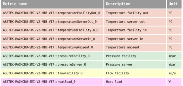
Cooling System
DAVIDE has three racks consisting of 15 compute-nodes each and an in-dependent Asetek RackCDU liquid cooling system mounted on each rack. The metrics recorded for these components are detailed in Figures 3a and 3b [13]:
3.2
Power Supply
ExaMon also keeps track of the LiteOn PSUs which supply power on each rack on the HPC system. Figure 4 lists the metrics recorded for these com-ponents:
3.3
Intelligent Platform Management Interface
Intelligent Platform Management Interface (IPMI) is a hardware-based so-lution used for securing, controlling, and managing servers. Many metrics related to the IPMI are monitored by ExaMon for each compute-node. The metrics recorded for these components are listed in Figure 5:
3.4
On-Chip Controller
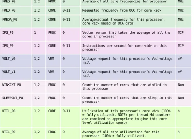
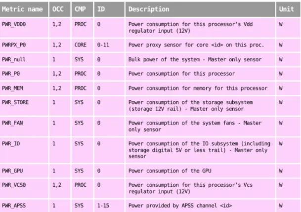
The On-Chip Controller (OCC) is a co-processor embedded directly on the main processor die. It can be used to control the processor frequency, power consumption, and temperature in order to maximize performance and minimize energy usage. Figures 6a, 6b and 7 detail the metrics recorded for these components:
The metrics listed in the figure below describe the per-component power consumption:
Figure 7: On-chip controller metrics.
3.5
Fine-grained Power
Power consumption at compute-node power plug is recorded with a sam-pling rate of 1ms. This metric generates a huge amount of data in compar-ison to the aforementioned metrics, which have a sampling rate of 5 or 10 seconds.
Figure 8: Fine-grained power metric.
A total of 160 metrics are monitored, but the number of metric param-eters is significantly higher. For instance, each of the metrics that contain per-core measurements can be divided into 12, one for each of the 12 cores in each On-Chip Controller monitored.
4
Password Cracking Activities
In order to simulate anomalous activity, multiple password cracking jobs were run simultaneously. Since the use of existing offline password crack-ing software such as Hashcat or John the Ripper would probably have alerted system administrators, leading to my account being blocked, a simpler al-ternative was adopted.
The goal was to collect the hardware metric data generated by pass-word cracking activities in the HPC system. Therefore two scripts were created, one implementing a brute force attack (a technique employed in both password cracking and crypto-mining) and one simulating a dictio-nary password attack.
Both scripts were kept as simple as possible so as to avoid detection by the current malware detection system, while allowing me to collect the HPC system’s hardware component data. If a machine learning model were to successfully identify a set of common instructions (such as nested for-loops) as anomalous, detecting more specific and unique behaviours would be straightforward.
Again, it must be emphasized that the task was to collect the data gen-erated by the HPC system while performing a specific activity, in order to discriminate it from the others. The goal was not to identify state-of-the-art advanced password cracking algorithms running on the system, but rather to build a learning model capable of classifying a specific collection of jobs based on the data generated by the hardware components.
On the following days: 23/12/2019, 24/12/2019, 27/12/2019, 28/12/2019, 29/12/2019, 30/12/2019, 31/12/2019, 08/01/2020, 09/01/2020, 10/01/2020, 76 anomalous jobs were run on the system. Half were brute force attacks, half dictionary attacks.
Some of them were run on a single node, while others on two nodes. Some engaged all available resources in the node(s), while others shared the computational power with multiple jobs running on the same node(s). This allowed us to collect sensor data from the HPC system while running
under different conditions.
4.1
Brute force attack
Algorithm 2Password cracking: brute force attack password ⇐ read first argument
if password is empty then
password = random_password(length=random_length([3 . . . 6])) password = hash_password(password)
for len in [1 . . . 6] do
for guess in len long combinations of chars and digits do if hash_password(guess) = password then
return true return false
The brute force attack script is simple and its pseudo-code is shown in Algorithm 2. The script can receive a generic string (i.e. a plain-text password) as argument. If no string is passed as input, then a random ASCII string composed of characters and digits is generated. The string is then hashed using the bcrypt library [14], an implementation of the Blow-fish cipher, which is the standard hashing algorithm for many operating systems, such as OpenBSD and SUSE Linux.
Finally, we generate all possible character and digit combinations of a variety of lengths, ranging from 1 to 6. If a matching password is found, the execution ends.
4.2
Dictionary attack
Algorithm 3Password cracking: dictionary attack mpos ⇐ read first argument
password ⇐ read second argument
if password is empty then
password = random_password(length=random_length([3 . . . 6]))
else if password = ’random’ then
password = get_random_word(’passwords.txt’, max_pos=mpos) password = hash_password(password)
for index, psw in ’passwords.txt’ do if index < mposthen
if hash_password(psw) = password then return true
else break return false
Dictionary attacks usually rely on a list of common passwords in order to crack a given hash. The script works with the text file ‘passwords.txt’ which contains the 1,000,000 most common passwords according to Se-cLists [15].
The script can either draw a password at random from ‘passwords.txt’, receive a plain-text password as input or generate a random sequence of characters and digits. In the latter case the password will probably not be found during the dictionary attack, however it is useful to collect system data regarding this scenario also. The plain-text password is then hashed with the same cipher used in the brute force script.
Finally, the script loops over all the passwords in the dictionary. The user can also specify a maximum number of attempts as argument. If a matching hash is found or the number of attempts reaches the specified value, the execution ends.
5
Feature Selection
As described in Chapter 3, ExaMon monitors a variety of physical and architectural components, which results in many hundreds of metrics be-ing recorded. However, trainbe-ing a machine learnbe-ing model with such an amount of features could put unnecessary computation burden on the model, reducing generalization and increasing overfitting.
Therefore, feature reduction by means of selecting few valuable met-rics is desirable. As previously seen, the recorded metmet-rics describe very heterogeneous hardware components (cooling system, power supply, on-chip controllers, and so on) and record data in many different units of measurement (Celsius, Volt, Ampere, Watt, percentages, and so on). In this context it is preferable to let the end user choose which architectural metrics to use to detect anomalous activities according to their knowledge of the HPC system.
In order to select the metrics to use for our study we relied both on our knowledge of DAVIDE and on the insights provided by a statistical analysis of the data. We computed the Principal Component Analysis [16] in order to determine which linear combinations of metrics contain the larger amount of "information", and we used these insights to support the metric selection process.
5.1
Principal Component Analysis
Principal Component Analysis (PCA) is a technique used to reduce the dimensionality of large datasets, increasing interpretability while at the same time minimizing information loss. This method achieves these re-sults by creating new uncorrelated variables that successively maximize variance.
This chapter provides a brief overview on the intuition behind PCA and how we took advantage of it to select our metrics.
5.1.1
Standardization
Standardization is a preprocessing technique which aims to standardize the range of the initial continuous variables so that each one of them con-tributes equally to the analysis.
PCA is quite sensitive to the variances of the initial variables. In fact, variables with larger ranges dominate over those with smaller ranges (e.g. a variable that ranges between 0 and 100 will dominate over a variable that ranges between 0 and 1), which may lead to biased results. Therefore, scal-ing the data to comparable scales can prevent this problem. Oftentimes, the difference in data ranges is caused by the adoption of different units of measurement (Ampere, Volt, Celsius, percentages, etc.), as is the case with our data.
The Z-score is one of the most popular methods to standardize data, and it consists in subtracting the mean (µ) from each value (v) and divid-ing the result by the standard deviation (σ), as shown in the followdivid-ing equation:
z= v−µ
σ .
Once the standardization is completed, all the features have a mean of zero, a standard deviation of one, and thus the same scale.
5.1.2
Covariance Matrix
A covariance matrix is computed in order to underline how the features of the input dataset vary from the mean with respect to each other. In other words, to determine the relationship that exists between them. As a matter of fact, features are sometimes highly correlated in such a way that they contain redundant information.
A covariance matrix is a symmetric matrix whose entries are the covari-ances associated with all the possible pairs of initial features. For instance, given the n×p sample matrix S, the variables X1, X2, . . . , Xprepresent the
The covariance matrix is a p×p matrix of the form C = Cov(X1, X1) . . . Cov(X1, Xp) .. . . .. ... Cov(Xp, X1) . . . Cov(Xp, Xp) .
In statistics, the covariance is a measure of the joint variability of two variables. The sample covariance between two variables A and B can be computed using the following formula:
Cov(A, B) = ∑
n
i=1(Ai−A¯)(Bi−B¯)
n ,
where Aiis the i-th element of the sample for variable A, ¯A is the
sam-ple mean for A, Bi is the i-th element of the sample for variable B and ¯B
is the sample mean for B. The covariance matrix can also be represented using matrix operations:
C =STS N−1.
Since the covariance of a variable with itself is its variance (Cov(a, a) = Var(a)), the main diagonal of the covariance matrix (top left to bottom right) contains the variances of each initial feature. Moreover, since the covariance is commutative (Cov(a, b) = Cov(b, a)), the entries of the co-variance matrix are symmetric with respect to the main diagonal, which means that the upper and the lower triangular portions are equal.
If the covariance between two features is positive, then these features increase or decrease together (i.e. they are correlated). Otherwise if the covariance is negative, then the two features move in opposite directions (i.e. they are inversely correlated).
5.1.3
Principal Components
Principal Components (PC) are new uncorrelated features that are con-structed as linear combinations of the initial features. They are concon-structed in such a way that most of the information contained within the initial fea-tures is "compressed" into the foremost components.
The principal components can be seen as the axes that provide the best angle to see and evaluate the data, such that the differences between the observations are best visible.
There are as many principal components as there are features in the data. Principal components are constructed so that the first PC accounts for the largest possible variance in the dataset. The second PC is computed in the same way, with the condition that it be uncorrelated with (i.e. per-pendicular to) the first principal component and that it account for the next highest variance. This process continues until a total of p principal components have been computed, equal to the original number of initial features.
Figure 9 shows a visual example of principal components in a 2 dimen-sional dataset.
Eigenvectors and eigenvalues of the covariance matrix C are computed in order to determine the principal components of the data.
The eigenvectors of the covariance matrix are the directions of the axes where there is the most variance (most information), called principal com-ponents. Eigenvalues are the coefficients attached to eigenvectors, which give the amount of variance carried in each principal component.
In order to find the eigenvalues of the covariance matrix C, the follow-ing equation must be solved:
det(C−λI) = 0,
where I is the identity matrix. The solutions to the equation above are the eigenvalues λ1, λ2, . . . , λp of the covariance matrix. The rank p of the
matrix determines the equation degree, which is equal to the number of eigenvalues.
Finally, in order to compute the eigenvectors of the correlation matrix C, the following equation must be solved:
C ¯xi =λi ¯xi,
where λi is the i-th eigenvalue of matrix C and ¯xi = [x1, x2, . . . , xp]T is
a column vector which represents the i-th eigenvector of the correlation matrix.
The result is a p×p matrix P, where the rows are the eigenvectors of C and specify the orientation of the principal components relative to the original features. These vectors are usually sorted by their eigenvalues, which quantify the variance explained by each principal component.
5.1.4
Feature Importance
The components of each eigenvector are called loadings and they describe how much each feature contributes to a particular principal component. Large loadings (positive or negative) suggest that a particular feature has
a strong relationship with a certain principal component. The sign of a loading indicates whether a variable and a principal component are posi-tively or negaposi-tively correlated. An example is shown below:
PC1 PC2 feature 1 2.12 0.23 feature 2 1.37 −1.05 feature 3 −2.38 0.16 feature 4 1.42 0.02 expl. var. 0.59 0.33
In the example above, only the first two principal components are con-sidered, because together they account for 92% of the total explained vari-ance, whereas the two remaining PCs are not considered relevant enough to be taken into account. The first principal component is most related to features 3 and 1, while the second PC is most related to feature 2.
The loadings were taken into account during the metric selection pro-cess. We selected the metrics according both to our knowledge of the sys-tem and their statistical importance.
5.2
Data Processing
Performing PCA on the whole dataset would be unnecessarily resource-consuming. Therefore, the analysis was carried out on data from four days in December: 09/12/2019, 22/12/2019, 28/12/2019 and 30/12/2019, Which represent about 10% of the whole dataset.
The script split_metrics_data.py creates a CSV file for each available metric. Each file contains one or more columns depending on the type of recorded data. For instance, metric "TEMP_P0", which records proces-sor and core temperatures, logs data from 2 different On-Chip Controllers (CMP=PROC and OCC=1,2) and from 12 cores for each OCC (CMP=CORE, OCC=1,2 and ID=0-11). Therefore, a total of 26 data columns are created: 12 columns for core ids 0 to 11 in OCC 1, 12 columns for core ids 0 to 11 in OCC 2 and two more columns for average processor temperature for OCC 1 and OCC 2.
each metric created with the script described above, in order to create a single CSV file. During the merging process, some data preprocessing was carried out. For instance, the metrics "CPU_Core_Temp_*", "DIMM*_Temp" and "Mem_Buf_Temp_*" were merged together by averaging the column values. The same was done for processor and core measurements (divid-ing by CMP: CORE and PROC). This preprocess(divid-ing is useful in reduc(divid-ing the number of features that are related to the same architectural metrics.
Finally, the script perform_pca.py performs the Principal Component Analysis using the Python library scikit-learn [17]. The resulting CSV file contains the principal components sorted by explained variance.
5.3
Selection of Relevant Metrics
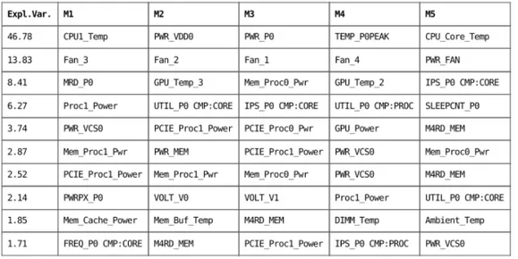
As mentioned before, the resulting file contains the principal components sorted by explained variance. For each component we list its loadings. That is, the degree of contribution of each metric to the principal compo-nent.
Figure 10: First 10 principal components and their first 5 metrics, sorted by highest-to-lowest loading values.
Figure 10 shows the 5 metrics that are most related to each of the first 10 components. The metrics selected for the anomalous activity detection described in the next chapters are listed in Table 3:
Metric PC Description Unit
CPU1_Temp 1 IPMI package temperature ◦C PWR_VDD0 1 Power consumption for Vdd regulator W PWR_P0 1 Processor power consumption W
Fan_3 2 Fan 3 speed RPM
Fan_2 2 Fan 2 speed RPM
MRD_P0 3 Memory read requests per sec. GB/s Proc1_Power 4 CPU power consumption W PWR_VSC0 5 Power consumption for Vcs regulator W Table 3: Metrics selected for the anomalous activity detection. These metrics provide a general overview of the system state by con-sidering different measures like power consumption, IPMI temperature, fan speed, memory requests, and so on. We do not apply the PCA to the whole dataset and use the resulting variables in the analysis because we want the learning model to detect anomalous activities using initial fea-tures as they are delivered by the monitoring framework. Thus, no extra expensive computations are required in potential real-world applications.
6
Temporal Convolutional Networks
Temporal Convolutional Network is a relatively new deep learning archi-tecture which has shown significant results in processing time series data. For this reason, it is employed in this thesis to discriminate between nor-mal and anonor-malous activities.
The data collected by ExaMon model the state of the HPC system by inspecting many physical and architectural metrics. These temporal se-quences of sensor data form multivariate time series, which are submitted to a Temporal Convolutional Network with the aim of identifying anoma-lous activities.
For time series analysis, the most commonly used technologies are Recurrent Neural Networks (RNN). Derived from feed-forward neural networks, RNNs can use their internal state, called memory, to process variable-length sequences of inputs. However, the basic RNN model is generally not directly suitable for computations requiring long-term mem-ory; rather, a RNN variant known as Long Short-Term Memory (LSTM) is usually employed. LSTMs can process sequences with thousands or even millions of time points, and have good processing abilities even for long time series containing many high (and low) frequency components [18].
However, the latest research shows that the Temporal Convolutional Network (TCN) architecture, one of the members of the Convolutional Neural Network (CNN) family, shows better performance than the LSTM architecture in processing very long sequences of inputs [19]. A TCN model can take a sequence of any length as input and output a processed sequence of the same length, as is the case with an RNN. Moreover, the convolution is a causal convolution, which means that there is no informa-tion "leakage" from future to past.
TCNs use a one-dimensional, Fully Convolutional Network (1D FCN) architecture to produce an output of the same length as the input. Namely, each hidden layer is zero-padded to maintain the same length as the in-put layer. To avoid leakage from future to past, a causal convolution is
adopted, which means that an output at time t is the result of the convo-lution of exclusively elements from times t or earlier in the previous layer [20].
6.1
Sequence Modeling
Sequence modeling is the task of predicting what value comes next. Given the input sequence x0, x1, . . . , xT, the task is to predict some corresponding
outputs y0, y1, . . . , yT at each time. In this context, the key constraint is that
to predict the output yt for some time t, only the inputs that have been
previously observed (that is, x0, x1, . . . , xt) can be used.
Formally, a sequence modeling network is any function f : XT+1 → YT+1that produces the mapping
f(x0, . . . , xT) = ˆy0, . . . , ˆyT,
while satisfying the causal constraint that yt depend only on x0, x1, . . . , xt
and not on any "future" input xt+1, xt+2, . . . , xT.
The goal of learning in a sequence modeling setting is to find a network f that minimizes some expected loss between the actual outputs and the predictions, L(y0, . . . , yT, f(x0, . . . , xT)), where the sequences and outputs
are drawn according to some distribution [21].
6.2
Fully Convolutional Networks
As mentioned above, a TCN makes use of a one-dimensional Fully Con-volutional Network architecture in order to produce an output sequence of the same length as the input.
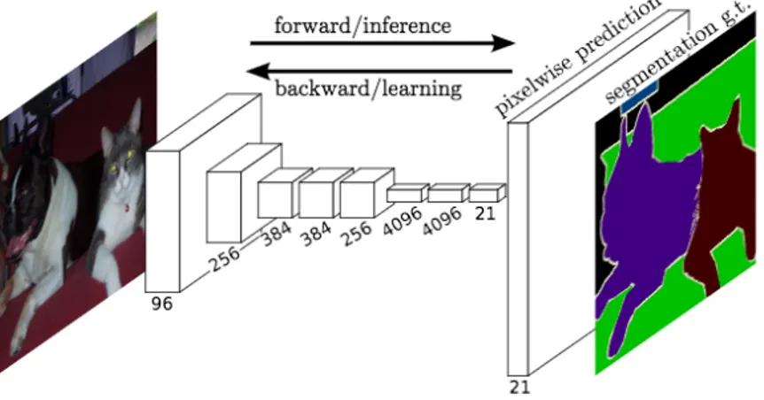
In an FCN, all the layers are convolutional layers, hence the name "fully convolutional". There are no fully-connected layers at the end, which are typically used for classification with a CNN. Instead, FCNs up-sample the class prediction layer and use a final convolutional layer to classify each value in a matrix (e.g. pixels in an image).
Therefore, the final output layer is the same height and width as the in-put matrix, but the dimension of each resulting cell is equal to the number of classes. Using a softmax probability function, the most likely class for each cell can be computed.
For instance, Figure 11 shows a 2D FCN used for image segmentation [22]. In the last layer each pixel is an N-dimensional vector with elements the probabilities of the image belonging to each class (which in the exam-ple are dog, cat, couch or background).
Figure 11: Example of image segmentation with an FCN.
Generally, TCNs make use of 1D FCNs which can process univariate time series data. However, if time series have multiple observations for each time step, the TCN can employ multi-dimensional FCNs.
6.3
Causal Convolutions
The second principle of TCNs is the absence of leakage from the future into the past. This is achieved by using causal convolutions.
Causal convolutions are a type of convolution used for temporal data which ensures that the model cannot violate the ordering in which the data is presented: the prediction yt emitted by the model at timestep t cannot
Figure 12: Example of causal convolutions in a network with 3 hidden layers.
Figure 12 illustrates which neurons each node of the output layer de-pends on.
6.4
Dilated Convolutions
A simple causal convolution is only capable of looking back at a history with size linear in the depth of the network. This makes it challenging to apply the aforementioned causal convolution on sequence tasks, espe-cially those requiring longer history. A solution is to employ dilated con-volutions that enable an exponentially large receptive field [21].
More formally, given a 1D sequence input x ∈ Rn and a filter f :
{0, 1, . . . , k−1} → R, the dilated convolution operation F on element s of the sequence is defined as
F(s) =
k−1
∑
i=0
f(i) ·xs−d·i,
where d is the dilation factor, k is the filter size, and s−d·i accounts for the direction of the past.
When d=1, a dilated convolution is identical to a regular convolution. Using a larger dilation factor enables an output at the top level to depend on a wider range of inputs, thus effectively expanding the receptive field
of the Convolutional Network. There are, therefore, two ways to increase the receptive field of the TCN: choosing larger filter size k and increasing the dilation factor d [21].
Figure 13: Example of dilated convolutions. Thanks to the dilations, the receptive field is larger than the one in Figure 12.
Figure 13 shows an example of dilated convolutions with filter size k=2 and dilations d= [1, 2, 4, 8].
6.5
Residual Connections
Since the receptive field of a TCN depends on the network depth n as well as the filter size k and the dilation factor d, stabilization of deeper and larger TCNs becomes important.
Very deep neural networks are difficult to train because of the vanish-ing and explodvanish-ing gradient problems. In order to mitigate these issues, residual blocks and residual connections can be employed.
Residual blocks consist of a set of stacked layers, whose inputs are added back to their final output. This is accomplished by means of the so-called residual (or skip) connections [23].
A residual block contains a branch leading out to a series of transfor-mations F, whose outputs are added to the input x of the block. Usually an Activation function is applied to the resulting value, which produces
the residual block output:
o= Activation(x+F(x)).
This effectively allows layers to learn modifications to the identity map-ping rather than entire transformations, a choice which has repeatedly been shown to benefit very deep networks.
Figure 14 shows an example of the residual blocks used in TCNs. If input and output have different widths, an 1×1 convolution is added to ensure that the element-wise addition receives tensors of the same shape.
7
Minority Class Oversampling
When the class distributions in a dataset are highly imbalanced, data are said to suffer from the Class Imbalance Problem. In this context, many clas-sification learning algorithms have low predictive accuracy for the infre-quent classes. Various approaches may be adopted in order to solve this issue.
Undersampling is a technique which aims to balance the class distribu-tion of a dataset by removing observadistribu-tions from the majority class. This approach is preferable when the minority class contains a large amount of data, despite being outnumbered by the majority class.
Oversampling is a different approach which addresses the class imbal-ance problem by integrating the minority class with new observations. Some popular techniques are: Random Oversampling, which randomly duplicates the samples in the minority class. SMOTE (Synthetic Minority Over-sampling TEchnique), which generates synthetic samples based on nearest neighbours according to euclidean distance between data points in the feature space. ADASYN (Adaptive Synthetic), which generates new samples for the minority class privileging the data points that are harder to learn according to their position in the feature space.
During the period of time in which we stored the data monitored by ExaMon, a total of 2761 jobs were recorded: 86 of them were password-cracking jobs, which we consider anomalous in the context of this thesis, whereas 2675 were considered normal activities in this analysis.
This disproportion between the classes could adversely affect the ac-curacy of the model. In order to mitigate this issue we oversample the anomalous class. This chapter describes how the system sensor data were translated to time series and the technique we adopted to oversample the minority class.
7.1
Data Preprocessing
As detailed in Chapter 3, the monitoring framework records a large amount of sensor data. In addition, ExaMon stores job information such as start and end date, execution time, the nodes on which a job was running, the user who ran the job, the user’s project account and more. Thanks to these data we are able to pair sensor values with the jobs that were running on the system.
Algorithm 4 shows the pseudo-code for the preprocessing script, which disaggregates sensor data into single metrics which are combined to create a multi-dimensional time series for each job run on the system.
Disaggregating sensor data into multi-dimensional time series asso-ciated with the recorded jobs is crucial in order to correctly identify the anomalous jobs executed on DAVIDE instead of just anomalous states of the system.
First, the script retrieves the information available for all the jobs which ran on the specified day. Then the jobs which did not run on monitored nodes and those which ran for more than 8 hours are filtered out. The reason is that during the data collection period, ExaMon was only config-ured on the following 18 compute-nodes: 17, 18, 19, 20, 21, 22, 23, 24, 34, 36, 37, 38, 39, 41, 42, 43, 44, 45. Moreover, the maximum job execution time for standard users on DAVIDE was 8 hours, while jobs lasting longer were run by system administrators. Filtering out sysadmin jobs, which could run up to 12 hours, decreased the size of the resulting dataset and as a consequence it reduced the computational cost required to train the learning model.
When a job runs over multiple days, the time series construction is de-layed: the sensor data regarding the current day being processed is trans-lated to the job time series, while the rest of the series is completed when the next day’s sensor data is processed. This is done by saving the pend-ing job id on a file in the ‘old’ folder of the next day. Then, each time the script is run, it checks if any jobs were saved in the current day’s ‘old’
folder. If so, these jobs are also included in the processing.
Algorithm 4Time series generation
metrics ← read input{list of metrics to extract}
from_date ← read input{consider only jobs run in this date} job_info ← retrieve data for jobs run in from_date valid_jobs ← create dictionary
for job in job_info do
if job.nodes in MONITORED_NODES and job.duration < 8H
and job.nodes 6= ’login’ then for node in job.nodes do
valid_jobs[node].append(job)
if from_date/old folder is not empty then
old_jobs ← read jobs in from_date/old
for job in old_jobs do for node in job.nodes do
valid_jobs[node].append(job)
metric_data ← read metric data for selected metrics
for node in valid_jobs do
for job in valid_jobs[node] do
if job.end_date = from_date + 1 day then
write job to next day’s /old folder
ts_files ← open CSV files for each combination of: job.id, node, CMP, OCC and ID available for metrics
for data in metric_data[node] do for job in valid_jobs[node] do
if job was running in data.timestamp then
param_comb ← job.id+node+data.cmp+data.occ+data.id ts_files[param_comb].write(data.measurement)
save and close all ts_files
3, metrics have different parameters depending on their type (e.g. cooling system metrics can be grouped by rack id, on-chip controller metrics can be filtered by occ, cmp and core id, and so on). Therefore each metric pa-rameter is a distinct dimension in the output job time series. For instance, the metric "UTIL_P0" adds 26 different dimensions to the job time series: 1 for average utilization of the first processor (OCC=1, CMP=PROC), 1 for the second processor (OCC=2, CMP=PROC), 1 for each of the 12 cores in the first processor (OCC=1, CMP=CORE, ID=0-11) and 1 for each of the 12 cores in the second processor (OCC=2, CMP=CORE, ID=0-11). With this decomposition, the learning model can take into account all the fine metric parameters, and not just the high-level metric overview (i.e. the model can learn from any of the 26 parameters of UTIL_P0 instead of just from their aggrega-tion).
In Chapter 4 we said that 76 password-cracking jobs were executed, however from this Chapter on we will refer to 86 anomalous jobs. This in-crease is due to the preprocessing script, which splits a password-cracking job executed over multiple nodes into multiple anomalous time series. This distinction is necessary because from the point of view of the mon-itoring framework a job execution over different nodes is equivalent to multiple parallel and independent executions.
7.2
Existing Oversampling Techniques
The simplest technique employed for oversampling is Random Oversam-pling. This method requires to randomly select samples from the minor-ity class and duplicate them in order to increase the number of samples available. The more advanced approaches can be divided into three main groups: interpolation techniques, probability distribution-based methods and structure preserving approaches.
A popular oversampling technique based on interpolation is SMOTE (Synthetic Minority Over-sampling TEchnique). The main idea is to ran-domly interpolate synthetic samples between the feature vectors of two
neighboring data points in the minority class [24]. Another famous tech-nique is ADASYN (Adaptive Synthetic) which also generates new data by interpolating neighboring samples, but privileging those minority class data points which are surrounded by a large number of majority class sam-ples. The reason behind this choice is that these data points are considered harder to learn [25]. However, since these techniques take into account only the local characteristics of the samples and not their correlation over time, many random data variations can be introduced, weakening the in-herent interrelation of the original time series data.
RACOG and wRACOG are two probability distribution based tech-niques. These methods use the joint probability distribution of data at-tributes and Gibbs sampling in order to generate new minority class sam-ples. While RACOG selects samples produced by the Gibbs sampler based on a predefined "lag", wRACOG selects those samples that have the high-est probability of being misclassified by the existing learning model [26].
MDO (Mahalanobis Distance-based Oversampling) is an example of structure-preserving approach. This technique generates synthetic sam-ples having the same Mahalanobis distance from the considered class mean as the other minority class samples [27]. Another example is SPO (Struc-ture Preserving Oversampling), which generates synthetic minority sam-ples based on multivariate Gaussian distribution by estimating the covari-ance structure of the minority class and regularizing the unreliable eigen-spectrum [28].
A quite recent technique that should be mentioned is OHIT (Oversam-pling of High-dimensional Imbalanced Time-series), which generates the structure-preserving synthetic samples based on multivariate Gaussian distribution by using estimated covariance matrices [29].
All the aforementioned techniques have advantages and disadvantages. A common drawback is the lack of reliable and easily available libraries, or the unsuitability of such libraries for time series data. These approaches and the theory behind them are quite complex and their implementation from the ground up is beyond the scope of this thesis. For this reason
we developed an oversampling technique, inspired by Random Oversam-pling, which generates new samples that are similar, but not identical, to the minority class time series; this plays an important role in preventing overfitting. Standard oversampling techniques, including Random Over-sampling, are almost always designed for cross-sectional data. This often makes them unsuitable for time series data. We intend to address this de-ficiency by proposing a computationally inexpensive technique which can oversample time series data by generating synthetic series close in feature space and with a similar trend to minority class samples.
7.3
Proposed Oversampling Method
The main idea is to generate synthetic samples by randomly selecting mi-nority class time series that can act as guidance for generating new, similar series. This way the synthetic samples will be close to the original time se-ries in feature space and they will consist of similar — yet not identical — sequences of values. The technique can be divided into two main parts: producing new time series lengths and generating sequences of synthetic values.
7.3.1
Generating Synthetic Time Series Lengths
Time series in our dataset represent the architectural metric data which were recorded while the jobs were running on the system, therefore their length can vary significantly. In order to oversample this type of data we first need to generate the lengths of the soon-to-be synthetic samples. A naive approach would be to randomly sample new uniformly distributed lengths. However this solution may not generate a faithful representa-tion of the minority class, especially if this contains jobs of non-uniformly distributed lengths. To address this, we first compute the job length dis-tribution of the minority class, and then we randomly oversample similar lengths according to the original distribution.
All time series have a sampling rate of 5 seconds (those of 10 seconds are interpolated to 5 seconds) and the maximum execution time is 8 hours, therefore there could be 5760 possible different lengths. Since it is very in-frequent to find time series of identical lengths, we consider as similar time series whose lengths differ by a few minutes. Thus we split the set of pos-sible lengths in multiple "windows" which contain time series with similar lengths. We define the size of the windows as W. As a consequence, the total number of windows is N = 5750W . The j-th time series of length lj
be-longs to the i-th window if wi ≤lj <wi+W, where wiis the i-th window’s
shortest length, that is, i·W,∀i ∈ [0, 1, . . . ,(N−1)].
After the aforementioned aggregation we can easily compute a vec-tor v whose i-th element is the total number of time series belonging to the i-th window. Then we can compute the discrete distribution vector p which contains the percentage of time series for each window. Finally, we can randomly generate the lengths of the synthetic series according to the distribution p of the original time series lengths.
Figure 15: Original time series length distribution on the left, original (black) and synthetic (orange) time series lengths on the right.
Figure 15 shows on the left the distribution of time series lengths in the minority class, grouped by windows. The window size is W = 60, which means that jobs belonging to the same window differ by a maxi-mum of 5 minutes. The plot shows that many jobs have run for about 2